Int8 about machine learning

This post opens a series of short posts that discuss how to use many random walk vectors (vectors describing probability distributions of random surfer on a graph – like pagerank) to find homogeneous groups of objects in a dataset. The main idea here is to combine the existing work of many researchers into one method. The mathematics behind these ideas might be complex, but we will try to be as ELI5-oriented as possible – so anyone can read, understand (at least basic bits) and implement it himself/herself. As the whole thing here relies on components that exist on different abstractions levels we will start from basic atomic terms that will later be enclosed in a building blocks for the final solution.

We will start from explaining notion of similarity between objects. It is essential for many machine learning problems.

Among various similarity measures the most popular is euclidean distance (in fact it is dissimilarity measure – we will soon tranform it into similarity), it is a length of a line segment between two points in euclidean space spanned by object features dimensions. Euclidean distance aggregates similarities between each of the features. It is defined as follows:

\[
d(a,b) = \sqrt{\sum_{i}^{D} (a_{i} – b_{i})^2}
\]

If two objects do not differ at any of the dimensions euclidean distance is zero, otherwise it is a positive number. Distances between all objects in a dataset are usually expressed in a form of a matrix called distance matrix.

We will now take a closer look at one example of such distance matrix, we will then jump from dissimilarity to similarity transforming distance matrix into similarity matrix using parametrized gaussian similarity function. Our main goal will be to find out how to compute similarity matrix – structure that encodes similarities between all objects in our dataset. We will also point out all difficulties that emerge while composing it.

Julia package named Distances is worth mentioning now. Lets install it and start looking into distance matrix based on iris dataset (we assume each column of a data matrix is a single observations and each row represents single feature)

#Pkg.add("Distances")
#Pkg.add("RDatasets") - datasets source

using Distances
using RDatasets 
iris = dataset("datasets", "iris")
data_matrix = transpose(convert(Array{Float64,2}, iris[:,1:4])) # transpose data frame is row oriented while pairwise computes distances between columns 
distance_matrix = pairwise(Euclidean(), data_matrix)

Just a quick marginal note on its speed. It is impressively fast. Try to compute distance matrix for 10000 objects, each having 10000 features.

data_matrix_big = randn(10000,10000);
@time pairwise(Euclidean(), data_matrix);
# elapsed time: 13.350062394 seconds (800880240 bytes allocated, 1.11% gc time)

(checkout the benchmarks for details)

We can now visualize iris dataset distance matrix using Gadfly visualization package

# Pkg.add("Gadfly") - install if not present 
using Gadfly
spy(distance_matrix)

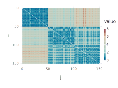
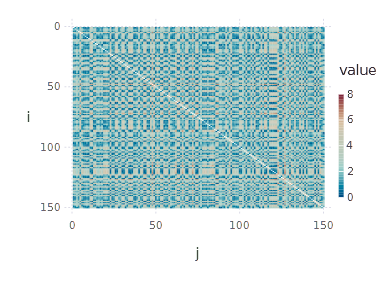
Lets try to interpret what we see. First of all indices \(i\) and \(j\) are indices of objects/observations, then upper left blue square visible on a distance matrix heatmap represents group of objects similar to each other (and not similar to other objects). Of course this is exceptional as our objects are sorted with respect to class memebership so basic cluster structure is visible. If we now shuffle the objects resulting plot will lose such expressiveness

shuffled_data_matrix = data_matrix[:,shuffle([1:size(data_matrix,2)])]
shuffled_distance_matrix = pairwise(Euclidean(), shuffled_data_matrix)
spy(shuffled_distance_matrix)

As you already notice the euclidean distance value reflects dissimilarity between objects, while we need similarity measure. Therefore we need a way to go from distance measure to similarity measure such that similarity = 0 reflects no similarity while similarity = 1 means practically same objects (up to features they are represented with).

The common way of achieving so is to apply the following function called Gaussian similarity function

where \(d\) is distance between considered objects. Lets see how it looks depending on choice of \( \sigma \).

function gaussian_similarity(sigma)
  return x -> exp((-x^2)/(2*sigma^2))
end 

yvalues = Scale.y_continuous(minvalue = 0, maxvalue = 1); 

plot(gaussian_similarity(.5), 0, 50, xlab , ylab, yvalues, Guide.title("sigma = 0.5"))
plot(gaussian_similarity(2.), 0, 50, xlab , ylab, yvalues, Guide.title("sigma = 2.0"))
plot(gaussian_similarity(5.), 0, 50, xlab , ylab, yvalues, Guide.title("sigma = 5.0"))
plot(gaussian_similarity(9.), 0, 50, xlab , ylab, yvalues, Guide.title("sigma = 9.0"))

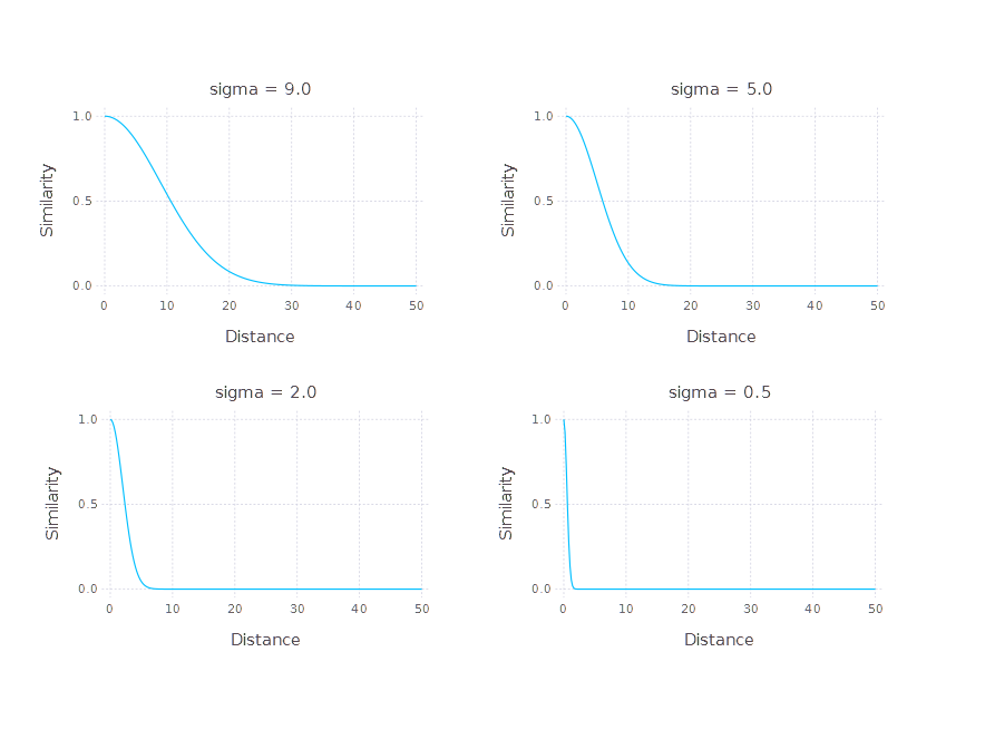
\( \sigma \) parameter can be seen as a soft threshold parameter on a distance value. In fact it is parameter controlling width of the gaussian function on positive part of \( \mathcal{R} \) domain. Anyway, transforming distance into similarity introduces problem of \( \sigma\) choice. Lets take a look at distance matrices of iris tranformed by gaussian similarity function element-wise (using different \( \sigma \) parameter) and corresponding histograms of similarities across whole dataset.

color_scale = Scale.color_continuous(minvalue=0,maxvalue=1);
sigma = 2;
similarity_matrix = map(gaussian_similarity(sigma), distance_matrix);
spy(similarity_matrix , color_scale);
plot(x = similarity_matrix[:], Geom.histogram);

Running the code above for different values of sigma results in the following outputs:

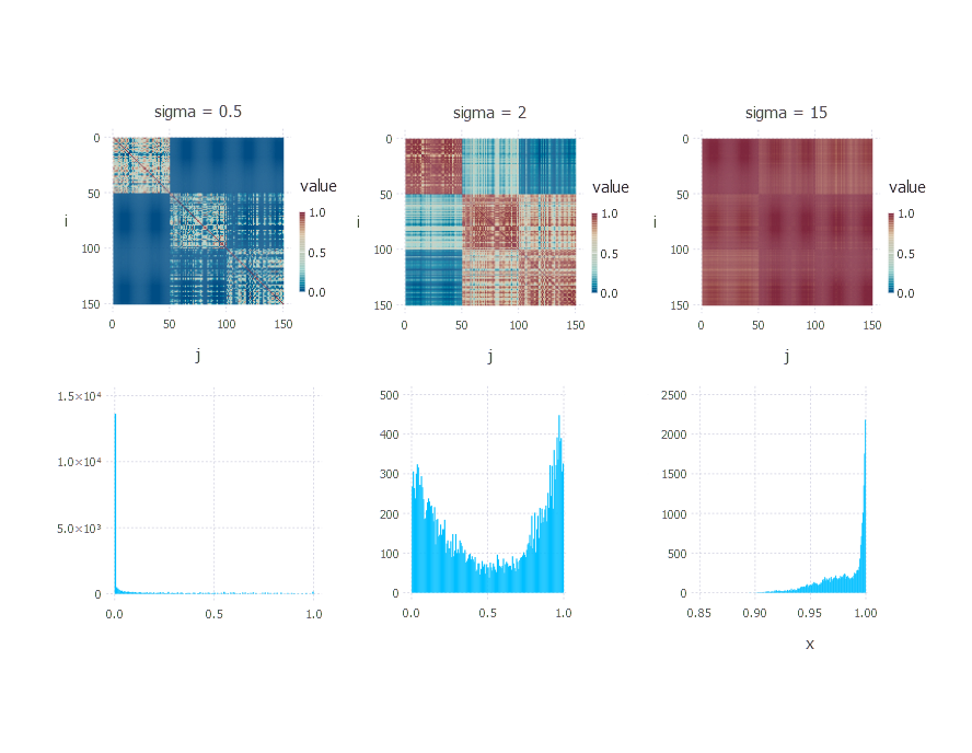
For different choices of sigma different matrices are produced with different distributions of values. The choice of sigma is crucial. If chosen sigma is too low then most of the similarity values are close to zero, if sigma is too high then all objects are very similar to each other with similarity close to 1. The choice of sigma is the problem itself and great care should be taken whenever distance matrix is tranformed into similarity matrix.

Summary

We presented one approach of how to represent and encode similarities between objects in your dataset. The problem of sigma choice was pointed out as crucial as it shapes the similarity matrix. We will keep it in mind and be careful when choosing sigma in the future.

Next post will cover one specific interpretation of the similarity matrix. The similarity matrix will let us think of our dataset as if it was a network with set of nodes and connections between them. This interpretation will be important for the main clustering problem (soon to be stated) we will try to solve.