Logistic Regression Part Ii Evaluation

This post is a continuation of a recent post where we implemented the gradient descent method for solving logistic regression problems. Today, we will try to evaluate our algorithm to find out how it works in the wild.

code

Last time, the logistic regression problem was stated strictly as an optimization problem, which suggests our evaluation should consider the goal function itself—which is to some extent correct; indeed, it makes sense to check how ( J ) changes while the algorithm runs. But it is not the best idea one can have. Please recall our goal. We aimed for a parametrized labeling machine producing labels for new upcoming observations/objects based on pre-defined features they are characterized by. The word new is crucial here. We want our model to fit to new data—to predict labels correctly for unseen data.

Therefore, we need some external metrics to measure how our model performs on data it does not know yet—in other words, we need to find out how well it generalizes. Generalization is the ability of a machine learning model to fit unseen data. The opposite phenomenon is called “overfitting”—it happens when a model predicts training data pretty well but fails on new upcoming examples—it learns patterns that are unique for training data omitting important general patterns that are common across the whole universe of possible objects of the given kind.

Our next steps are directed towards introducing external classification evaluation metrics, then building a logistic regression model for a chosen dataset (based on the code we already have), and applying these metrics onto it. In the meantime, we will also take a look at how ( J ) behaves over time (iterations).

Let’s begin then and present some basic terms around evaluation metrics for binary classifiers and list their pros/cons. We will also provide Julia implementation fitting the code we already have.

Confusion Matrix

A confusion matrix is a matrix (table) expressing classification results (class membership) with respect to true labels. Its column indices represent true classes while row indices represent classes assigned by the classification model. An entry of the confusion matrix reflects the number of objects falling into true-label/predicted-label categories. In our case, the confusion matrix is a square matrix of size 2.

One simple example, let’s say we deal with the problem of binary classification of text email messages into classes called “spam” and “not spam”. The following confusion matrix is then produced:

\[\begin{pmatrix} \color{green}{\text{[actual spam predicted as spam]}} & \color{red}{\text{[not spam predicted as spam]}} \\ \color{red}{\text{[actual spam predicted as not spam]}} & \color{green}{\text{[not spam predicted as not spam]}} \end{pmatrix}\]

Depending on where they land, observations falling into entries of the confusion matrix have the following names:

\[\begin{pmatrix} \color{green}{\text{[true positive]}} & \color{red}{\text{[false positive]}} \\ \color{red}{\text{[false negative]}} & \color{green}{\text{[true negative]}} \end{pmatrix} = \begin{pmatrix} \color{green}{\text{[TP]}} & \color{red}{\text{[FP]}} \\ \color{red}{\text{[FN]}} & \color{green}{\text{[TN]}} \end{pmatrix}\]

where positive indicates the email being spam, while negative indicates the email not being spam.

Let’s quickly implement confusion matrix calculation in Julia:

function confusion_matrix(predictions, labels, d)
   c = zeros(d, d)
   for i in 1:length(labels)
       c[labels[i] + 1, predictions[i] + 1] += 1
   end
   return c
end

And play with it:

labels = [x > 0.5 ? 1 : 0 for x in randn(1, 100)]
predictions = [rand(1)[1] > 0.1 ? labels[i] : (1 - labels[i]) for i in 1:100] # Let's miss the true target with prob 0.1 
confusion_matrix(predictions, labels, 2)

Resulting in something like (up to randomness):

\[\begin{pmatrix} \color{green}{\text{55}} & \color{red}{\text{9}} \\ \color{red}{\text{6}} & \color{green}{\text{33}} \end{pmatrix}\]

There are quite a lot of evaluation metrics that one can derive out of these 4 values (TP, FP, TN, FN). Let’s list, implement, and comment on the most important:

Accuracy

\[\text{accuracy} = \frac{TP + TN}{TP + TN + FP + FN} = \frac{\text{number of correct predictions}}{\text{number of observations}}\]

As described, it is quite a naive ratio of correct predictions. The main problem with such a metric is high dependency on class imbalance. For example, if we deal with 100 observations with 90 positive labels and our “classifier” classifies all new observations as “positive”, we land with accuracy = 0.9, which may indicate (at first glance) strong classification ability while our classifier is rather a toy.

Example Julia implementation below:

function accuracy(labels, predictions)
   sum(predictions .== labels) / length(labels)
end

Sensitivity

Also known as true positive rate or (recall) is defined as:

\[\text{sensitivity} = \frac{TP}{TP + FN}\]

Which is a ratio of correct predictions of positive labels and all true positive labels. In case of our spam/not spam example, that would measure how well we can predict spam (meaning, among all spam messages, how many of them we actually predict as spam).

Specificity

Also known as true negative rate is defined as:

\[\text{specificity} = \frac{TN}{TN + FP}\]

Which is a ratio of correct predictions of negative labels and all true negative labels. Again, in the case of our email example, it’s a way to measure how well we can predict “healthy” email (( TN + FP = ) number of all emails that are not spam).

Precision

Defined as:

\[\text{precision} = \frac{TP}{TP + FP}\]

Let’s think about that in the context of our email toy example. That is the ratio of the number of emails correctly predicted as spam to the number of emails predicted as spam—including incorrect predictions.

Once again, quickly, for training purposes, implement these metrics in Julia:

function sensitivity(predictions, labels)
    tp = 0
    fptp = 0.
    for i in 1:length(labels)
      if labels[i] == 1
          tp += predictions[i]
          fptp += 1.
      end
    end
    return tp / fptp
end

function specificity(predictions, labels)
    tn = 0
    tnfp = 0.
    for i in 1:length(labels)
      if labels[i] == 0
          tn += 1 - predictions[i]
          tnfp += 1.
      end
    end
    return tn / tnfp
end

function precision(predictions, labels)
    tp = 0
    fp = 0.
    for i in 1:length(labels)
      if labels[i] == 1
          tp += predictions[i]
      else
          fp += predictions[i]
      end
    end
    return tp / (tp + fp)
end

Having these pieces in place, it is probably high time to mention another “problem” that will motivate the last evaluation metric mentioned in this post. It is about the problem of choosing the proper threshold when dealing with models returning real values (like in the logistic regression case) instead of “labels” directly (KNN could be an example of such).

Let’s stick to logistic regression. Choosing the proper threshold is about what exactly should be considered a positive or negative prediction. Please recall that the logistic regression model crunches (transformed) input through a logistic function that returns values from the range ( (0,1) ). In other words, it does not return suggested binary labels. Then one must choose a threshold value that will serve as the minimum value for the model output to be interpreted as a positive prediction. Choosing one particular threshold results in a single classifier. Each choice implies specificity and sensitivity values. Now, if you consider all possible choices of threshold, you land with a set of 2-dimensional points in sensitivity-specificity space. These points draw a curve. The curve is called the ROC curve.

ROC Curve

Different ROC curves exist; here we will talk about one particular, the one in specificity/sensitivity space. The ROC curve is then defined as a set of points in ( \mathcal{R}^{2} ) where each point is defined as

\[\left( 1 - \text{specificity}(\mathcal{M(t)}, X_{\text{test}}), \ \text{sensitivity}(\mathcal{M(t)}, X_{\text{test}}) \right)\]

where ( \mathcal{M(t)} ) is a model under consideration for chosen threshold ( t ) and then sensitivity and specificity are calculated for the given model and test set ( X_{\text{test}} ). First of all, as the range of possible values for sensitivity and specificity is ( (0,1) ), the ROC curve exists in a unit square. Let’s take a look at the example of the ROC curve for a logistic regression model on the iris dataset with target = “versicolor” (on the training dataset).

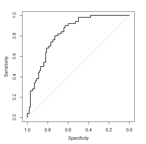
And comment on the border points:

• The upper right point has sensitivity = 1 and specificity = 0. It is the point with threshold = 0 implying a classifier that always returns positive predictions. Therefore, the true positive rate (sensitivity) is 1 as all predictions are positive, and the true negative rate (specificity) is 0 for the same reason.
• The bottom left point has sensitivity = 0 and specificity = 1. It is the point with threshold = 1 representing a classifier that always returns negative predictions. Analogically, the true positive rate (sensitivity) is 0 as all positive cases are predicted incorrectly, and the true negative rate (specificity) is 1 as all predictions are negative predictions.

Points in between represent classifiers resulting from choosing thresholds from ( (0, 1) ).

How will the ROC curve look for a potentially ideal classifier, the one for whom exists a threshold that perfectly separates observations? For that particular perfect threshold, it will generate specificity and sensitivity equal to 1 with lower values for other thresholds. The final ROC curve will look like this:

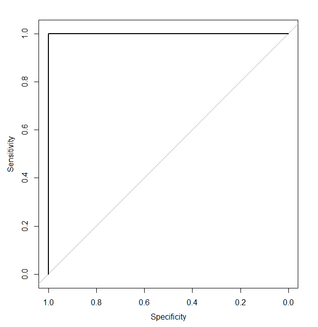
To wrap ROC curve information into a single metric, people use something called AUC – Area Under the Curve, which is a very common practical metric for classifier performance. AUC around 0.5 implies a purely random classifier, while AUC equal to 1 implies a perfect one.

If you want to get deeper insight into presented topics, take a look at Elements of Statistical Learning where PDF version is available.

Let’s try to implement AUC calculation in Julia. Our required input is a vector of labels (binary) and a vector of predictions (real). The main trick here is to sum up areas of consecutive triangles made of: point ( (1, 0) ), ( i )-th ROC curve point and its ( (i+1) )-th point. We will then need to identify all possible thresholds, iterate through these thresholds, compute the current triangle area, and sum these areas up to produce the final result.

Let’s try to write some code:

function triangle_area(A, B, C)
  0.5 * abs((A[1] - C[1]) * (B[2] - A[2]) - (A[1] - B[1]) * (C[2] - A[2]))
end

function auc(labels, predictions)
   n = length(labels)
   ROC_curve_points = ones(n+1, 2)
   sorted_labels = labels[sortperm(predictions)]
   prev_point = [1., 1.]
   total_auc = 0.
   predicted_labels = ones(n)
   for i in 1:n
     predicted_labels[i] = 0
     A = [1 - specificity(predicted_labels, sorted_labels), sensitivity(predicted_labels, sorted_labels)]
     ROC_curve_points[i, :] = A
     B = prev_point
     C = [1, 0]
     total_auc += triangle_area(A, B, C)
     prev_point = copy(A)
   end
   return ROC_curve_points, total_auc
end

The triangle_area function computes the triangle area using the Shoelace formula. The auc function first sorts labels with respect to predictions, then it sets all predictions to 1. At each iteration, the current permuted label is set to 0, and for such a prediction point, ( A ) is computed. Then, finally, the area is updated by the current triangle area given by the last point, the current point, and the point ( [1, 0] ). Moreover, ROC curve points are returned for later visualization.

The code is not so optimal—just note that specificity and sensitivity are computed separately at each iteration making the whole calculation of inefficient quadratic time. Optimal code should involve calculating all sensitivity and specificity values in one function cleverly relying on results from previous iterations. I will try to add this to the code on GitHub—as soon as it happens, you won’t see this remark.

Cross Validation

Okay, let’s gather all pieces together. We know how to build a logistic regression model, we know it tries to minimize a certain goal function, and we know how to compute AUC to evaluate the model. What we still miss is a way of dataset division into training and test sets—to evaluate generalization ability. A common way is to divide the dataset into ( K ) chunks—build the model ( K ) times, each time using one chunk as a test set for evaluation. This technique is called k-fold cross-validation.

We will now propose a simple implementation of k-fold cross-validation and comment on it right after.

function cross_validation(k, learn_method, dataset, labels, evaluation_metric)
 n = size(dataset, 1)
  if n < k
     error("Number of folds is greater than number of observations")
  end
  # Shuffle dataset
  shuffled_indices = shuffle([1:n])
  # Divide dataset into k chunks
  fold_cardinality = div(n, k)
  fold_indices = [[(fold_cardinality *(i-1) + 1):(fold_cardinality *i)] for i in 1:k]
  # Add missing observations to the last chunk
  fold_indices[end] = fold_indices[end][end] < n ? vcat(fold_indices[end], (fold_indices[end][end]+1):n) : fold_indices[end]

  f = learn_method[:learning_method]
  predict = learn_method[:inferencer]
  params = learn_method[:params]

  predictions = zeros(n)
  goal_function_values = []
  for fold in fold_indices
      test_indices = shuffled_indices[fold]
      training_indices = filter(a -> !(a in test_indices), shuffled_indices)
      training_dataset = dataset[training_indices, :]
      training_labels = labels[training_indices]

      model_params, goal_function_values = f(training_dataset, training_labels, params)

      test_dataset = dataset[test_indices, :]
      predictions[test_indices] = predict(test_dataset, model_params)[:]
  end

  return predictions, evaluation_metric(labels, predictions), goal_function_values
end

The main idea here is to:

• Iterate through subsets of shuffled indices (data matrix rows)
• Use these subsets as test data and the remaining elements as training data
• Each time produce the model using the selected learning method (in our case logistic_regression_learn function) and learning parameters
• Each time store the predictions for the given indices subset
• Having all predictions, evaluate them using the chosen evaluation metric (in our case auc function)

Real World Example

Well, it is not really a real-world example because the dataset we are going to examine is quite ‘easy’ to separate. It does come from the real world though. We are going to work with a dataset called “breast cancer”. It consists of 699 cases described by 10 attributes each. You can read a detailed description of the dataset here.

Okay, first of all, you can get the whole code that was created around logistic regression posts from the GitHub repository here.

include("LogisticRegression.jl")
include("Evaluation.jl")

# Pkg.add("RDatasets") - install RDatasets if you haven't already
# Pkg.add("Gadfly") - install Gadfly for visualization purposes
using RDatasets
using Gadfly

biopsy  = dataset("MASS", "biopsy")
median_of_missing_V6 = int(median(biopsy[:V6][!isna(biopsy[:V6])]))
biopsy[:V6][isna(biopsy[:V6])] = median_of_missing_V6
data = convert(Array{Float64, 2}, biopsy[2:10])
labels = convert(Array{Float64, 1}, biopsy[:11] .== "benign")

params = Dict([:alpha, :eps, :max_iter], [0.001, 0.0005, 10000.])
learn_method = Dict([:learning_method, :params, :inferencer], [logistic_regression_learn, params, predict])
predictions, eval_results = cross_validation(10, learn_method, data, labels, auc)

plot(x = eval_results[1][:,1], y= eval_results[1][:,2], Geom.line, Guide.xlabel("1 - Specificity"), Guide.ylabel("Sensitivity"))

Let’s see. First, we include our previously written code. Then we prepare data input and labels, propose a learning method with proper params, set evaluation metric, and run cross-validation (choosing 10 folds). Finally, we plot the ROC curve that results in the following plot:

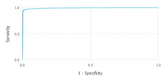
We can almost ideally separate points for a certain threshold. AUC is around 1. Let’s now pick one certain threshold, compute sensitivity and specificity, and comment on that. Let’s choose threshold = 0.5

sensitivity(labels, predictions .> 0.5)
0.9696312364425163

specificity(labels, predictions .> 0.5)
0.9537815126050421

As you can see, for that choice of threshold, we get very good performance of our classifier. Let’s think of that for a moment. What are the consequences of threshold choice taking into account the domain (potential breast cancer diagnosis) our classifier operates on? Of course, the loss of incorrect prediction in case of breast cancer is very high. It may result in the death of a patient. It differs from the opposite situation when we diagnose cancer for a healthy patient. Of course, it is extremely stressful for the patient, too. Losses of these decisions can be encoded in a structure called a Loss matrix—often provided by a domain expert. Then threshold choice minimizes the given loss.

There are still some unsolved mysteries around the code we just wrote. How does one know the alpha parameter? What should be the value of epsilon? When people don’t know but still want to look smart—they usually say it is rather an art than science. I’m gonna use that here. It is more an art than science, my dear friend. I honestly don’t know. But we can still empirically examine alpha choice. This time we can directly look at how the goal function changes over time. Let’s then experiment with alpha a bit and see how ( J ) changes over time (iterations)

params = Dict([:alpha, :eps, :max_iter], [0.00001, 0.005, 10000.])
results1 = logistic_regression_learn(data, labels, params)

params = Dict([:alpha, :eps, :max_iter], [0.0001, 0.005, 10000.])
results2 = logistic_regression_learn(data, labels, params)

plot(
     layer(x = 1:length(results1[2]), y = results1[2], Geom.line, Theme(default_color=color("red"))),
     layer(x = 1:length(results2[2]), y = results2[2], Geom.line, Theme(default_color=color("blue"))),
     Guide.XLabel("Iterations"), Guide.YLabel("J"),  Scale.x_continuous(minvalue = 0, maxvalue = 5000)
)

It produces:

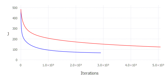
Choosing a smaller alpha results in slower convergence. On the other hand, choosing an alpha that is too large will not produce a good result, either. If the step size is too large, the algorithm will not have the flexibility to find the optimal solution—it will operate in a resolution that won’t let it find the optimal solution—it will finish iterating after max iterations—failing. The final conclusion is, you have to try out a few alphas, see how ( J ) changes—if it gets smaller without jumping around—it is probably okay. Another option is to experiment with adaptive gradient descent, where you don’t have to specify that parameter.

Summary

To summarize. I found implementing the gradient descent method for logistic regression problem quite convenient. It was fun. The main pain, though, I still experience is the lack of a good IDE. I also never established any mature workflow because of that. Right now, I still use REPL (console) and an external file in a text editor, which I think is a very basic approach.

Somewhere in the future, I will try to investigate what IDEs are out there and how to work in Julia in a correct and convenient way. See you soon!

---