My Adventure With Team Ball Action Spotting Task at SoccerNet Challenge 2025

In October 2024, a friend of mine asked me if I could help him with video processing problem of labeling soccer broadcasts with AI. I had absolutely zero knowledge about it though I promised I’d try do some research and share my findings so he has a starting point. This is how I learnt about SoccerNet - community of researchers focusing on soccer video analysis. Each year SoccerNet organizes SoccerNet Challenge that includes various tasks such as action spotting, camera calibration, player re-identification and tracking. When I learnt about it in late 2024 the challenge was about to start. I had one idle RTX 4090 GPU which was embarrassingly cold most of the time. I decided to give it a reason to run and started looking at one of the tasks: Team Ball Action Spotting Task.

Team Ball Action Spotting Task

The goal of Team Ball Action Spotting Task is to build a model that annotates soccer matches 90min videos with 12 different labels: Pass, Drive, Header, High Pass, Out, Cross, Throw In, Shot,Ball-Player Block, Player Successful Tackle, Free Kick, Goal. Additionally model has to predict the team that performs the action.

Team BAS SoccerNet Dataset

The training data consists of 7 densely annotated (around 2k annotations per match) soccer games + around 500 historical broadcasts (annotated via “old” seemingly irrelevant action labels). Our 7 densely annotated games are annotated via accompanied Labels-Ball.json file provided for each input video:

{
  "UrlLocal": "relative/fs/path/to/video.mp4",
  "UrlYoutube": "", // optional Youtube URL 
  "halftime": "1 - 46:04", // end of the first half 
  "annotations": [ // annotations list 
    {
      "gameTime": "1 - 00:00", // game time of the event (this is kick-off pass)
      "label": "PASS", // label of the event 
      "position": "680", // position in milliseconds 
      "team": "left", // team that performed the event
      "visibility": "visible" // visibility of the event (can be ignored)
    },
    // ...
  ]
}

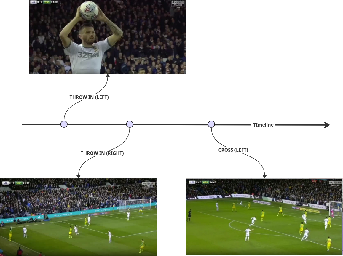
JSON file describes all events happening within one single match. The most important properties are “label”, “team” and “position”. They describe the type of event, its time-placement and the team that performed it.

Video together with accompanied labels file result in ~90 minut labelled timeline. A Single match has around 2000 events.

.

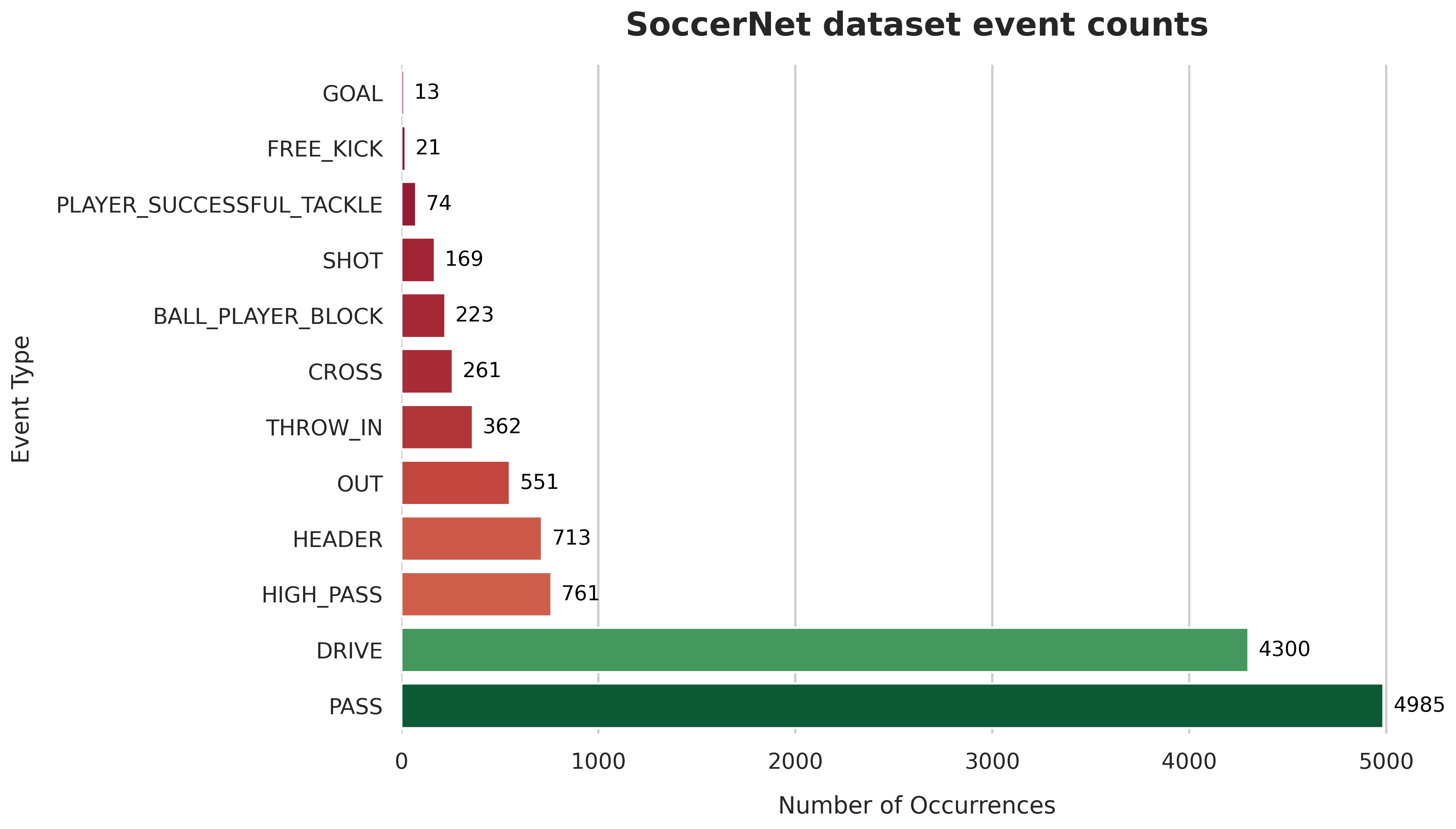
Event counts are distributed far from uniformly. The most common events are passes and drives while (unfortunately) goal is the rarest event happening only 13 times across whole dataset. The unbalanced nature of whole dataset is depicted below: .

Another problematic aspect of the training dataset is its very low variability. Dataset comes from 7 games only from a single league, therefore there is very limited variance in camera angle, lighting conditions, color of the field, t-shirt color, etc. This, if not addressed properly, may lead to overfitting.

Solution

Given little knowledge about the domain I decided to start simple and extend baseline model based on T-DEED by Artur Xarles - the winner of 2024 Action Spotting Challenge. Before starting the refinement of the baseline model I decided to invest a bit and implement data interface for Team BAS SoccerNet Challenge - this I hoped would make experimentation a bit faster + it would let me understand the dataset and its properties better by getting my hands dirty.

dude.k package

This is how I landed implementing dude.k - currently it contains data interface together with training/eval scripts + refined T-DEED model. You can install it via pip

pip install dude.k

I recommend following the README to learn a bit more about it. Long story short: it exposes the interface for accessing local file system videos, their annotations + bunch of routines to split videos into clips, access video frames (once extracted) and what not.

Refinement of the baseline model

Let’s take a look at the baseline T-DEED interface together to spot some low-hanging fruit. In inference time, T-DEED model consumes a clip (or multiple clips) consisting of N RGB frames and outputs bunch of predictions for each frame. Clip is a tensor of shape [N, 3, H, W] where N is the number of frames in the clip and the remaining dimensions represent single RGB frame.

Baseline T-DEED crunches the clip tensor and produces a bunch of predictions for each frame. These predictions in default “joint train” mode, include the following:

• team prediction head producing vector of size 3. Its values represents probability of left team performing action in given frame, right team or no team (in case of no action). Team prediction head is related to ball actions not “old” actions from historical broadcasts.
• ball action prediction head producing vector of size 13. Each index in a vector represents one of 12 possible actions or background.
• “old” action prediction head producing vector of size 18 (17 old classes + background)
• displacement head producing single scalar for each frame.

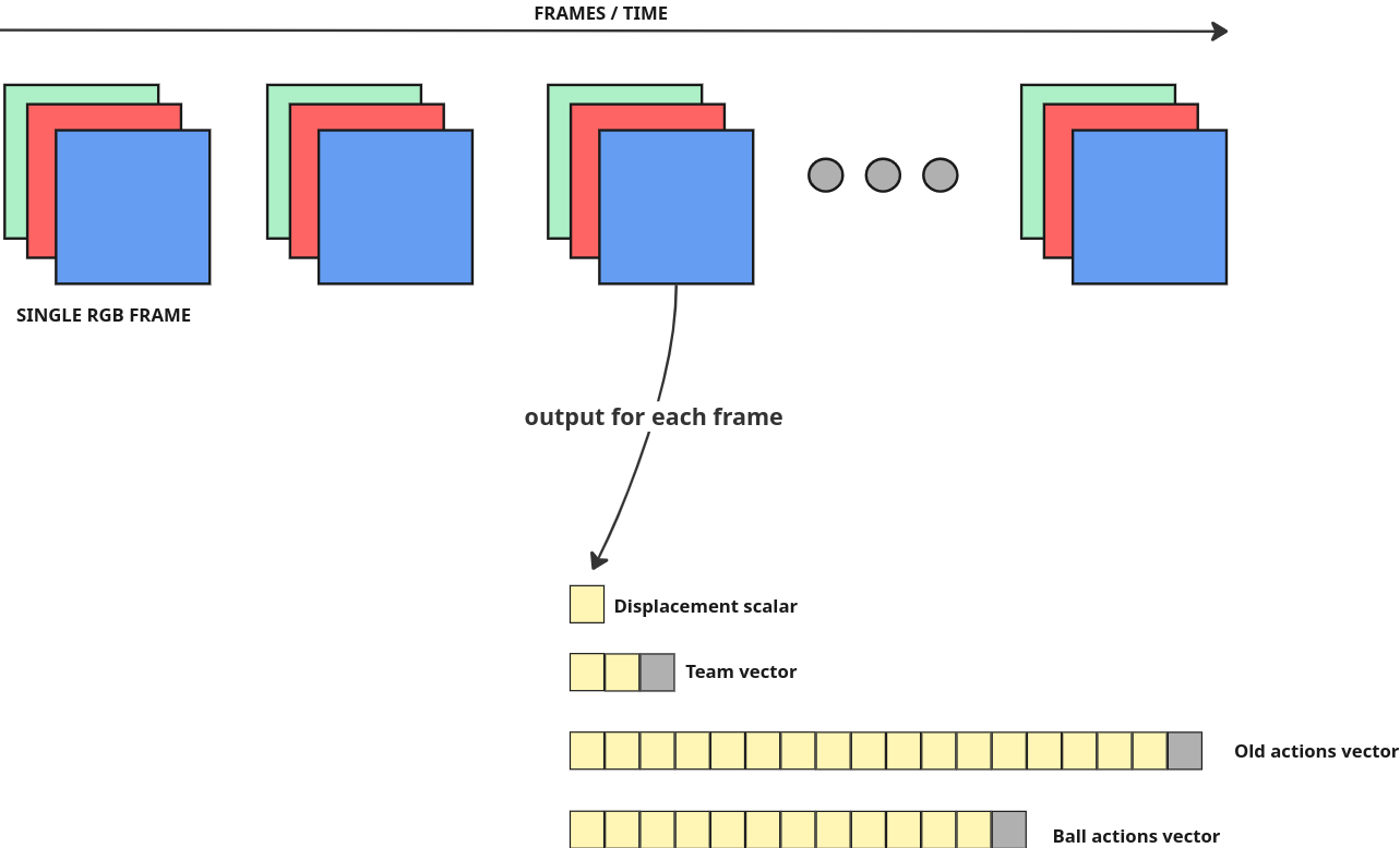
In simple terms then: For each clip of, let’s say, 200 frames (8 seconds with 25 fps) we will get 200 team predictions, 200 ball action predictions, 200 team predictions and 200 displacement scalars.

As you can already tell baseline model is trained on both “old” and “new” data. There is no separation between pretraining and fine-tuning but rather “joint” training of both predicion heads. Another bit that stands out and I believe makes baseline model training a bit harder is existence of team head as separate entity. There is some redundancy in there and it may be worth looking into.

This leads to the 2 major improvements over baseline model

• encoding team information into event labels.
• separation between pretraining and fine-tuning

Encoding team information into event labels

Baseline model outputs team information separately from ball action. Each frame is assigned to one of three values: left, right or none. Model therefore has to learn “no-action” information twice - for team head and for ball action head - which is already redundant. I decided to choose alternative approach and encoded team information into labels. So instead of predicting two separate values via two heads: team + ball action, I decided to melt team head and ball action head together. This way I’m able to learn “no-action” information once. Instead of 12 ball actions + single background (no action) vector my refined model outputs vector of size 12x2 + 1 instead. So instead of “action” alone and “team” alone I predict “action-team” cartesian product within one head.

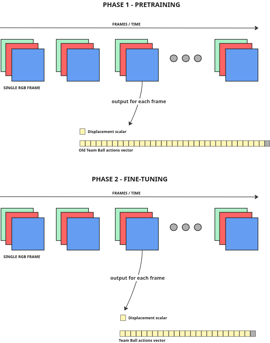
Separation between pretraining and fine-tuning

Another improvement I believed could be beneficial was separation between pretraining and fine-tuning. I therefore pretrain the model on “old” actions first (here I have 500 broadcasts at hand) and only then fine-tune on challenge 7 densely annotated videos.

Augmentations

As we already pointed out our training data is limited to 7 matches from one particular season and one league. Low variability of our data will lead to poor generalization of the model. Therefore we need aggressive augmentation strategy. Except of the baseline default augmentations I used the following ones:

Horizontal flip

The very first low hanging fruit is horizontal flip augmentation. It’s a simple but effective way to increase the number of training samples. Flipping a clip horizontally means flipping each frame and switching team information. Below you can see a clip before and after horizontal flip.

Crop

Another important augmentation I used is a random crop. I crop each frame at 90% of original size. Not that significant as horizontal flip but it is another way to increase the number of training samples. Example below:

Camera movement

Here, I use random frame rotation and translation to mimic camera movement of a broadcast. This is inspired by Ruslan Baikulov solution from 2023. Example below:

Pretraining / Fine-tuning

I kept original loss function composed of two components: the mean squared error (MSE) for the displacement head and a weighted cross-entropy for the team-x-label prediction. I set the foreground weight at 5, and weighted the loss components as follows: 1.5 for cross-entropy and 1.0 for the MSE.

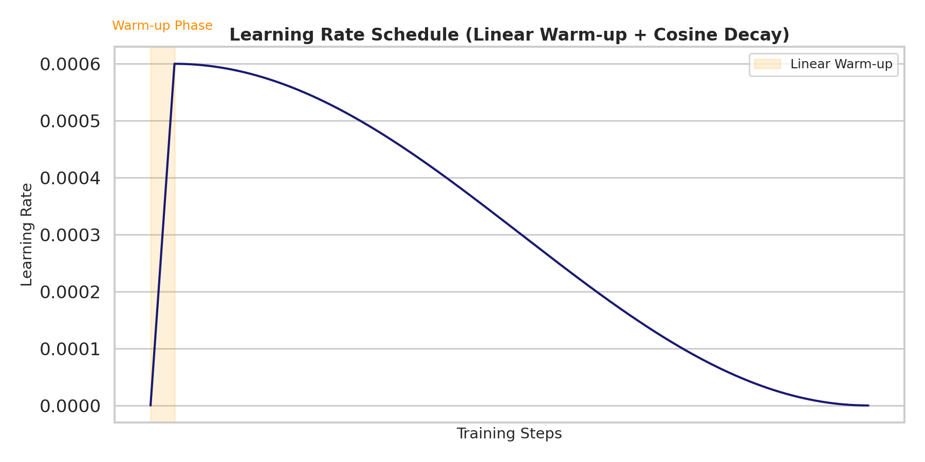
I used the AdamW optimizer, with a linear warm-up of one epoch followed by a cosine decay learning rate schedule. The initial learning rate was set to 0.0006, decaying down to 0 over 30 epochs.

My training data consisted of 5000 RGB clips per epoch, each with a length of 80 frames, an overlap of 68 frames between consecutive clips, and a spatial resolution of 224x224px. For both pre-training and fine-tuning, I used a batch size of 4.

During pre-training, my goal was to minimize the validation loss. For fine-tuning, I instead optimized mAP@1: the primary metric of the challenge. Additionally, I applied all my data augmentations with a probability of 0.2.

Input & Model	Value	Training & Post-processing	Value
Resolution	224x224	Optimizer	AdamW
Clip length	80	Learning rate	0.0006
Clip overlap	68	LR schedule	1 warmup + 29 cosine
T-DEED layers	2	Batch size	4
Displacement	4	Class weights	[5, 1]
SGP Kernel Size	5	Loss weights	[1.5, 1]
Backbone	regnety_008	Soft NMS window	34 frames
		Soft NMS threshold	0.005
Augmentations		Experiment
Horizontal flip	0.2	Pretraining data	500 broadcasts
Random camera movement	0.2	Fine-tuning data	7 Team BAS matches
Random crop	0.2	Validation setup	Train 4, val 1
		Final submission train	20 epochs, no val

Post-processing

Once the model is trained, we obtain a function that predicts a team-label at every frame of a given clip. If we just naively cut the initial 90-minute broadcast video into clips with no overlap and run inference, we’re technically done, but this approach isn’t optimal. Some clips prepared this way will not include enough surrounding context information. To address this, we run inference on overlapping clips. However, this introduces another issue: we may get multiple predictions clustered closely around a single event, negatively affecting our metric. We can address this challenge by employing Non-Maximum Suppression (NMS), keeping a single highest prediction per event while suppressing neighbors..

For our task, variation called Soft Non-Maximum Suppression (Soft-NMS) is used (already present in baseline), which reduces the scores of neighboring predictions instead of completely zeroing them out.

Soft-NMS approach uses two hyperparameters:

• score threshold: predictions with scores underneath this threshold are set to zero.
• class window: a temporal range (in frames) within which predictions scores are aggregated.

I optimized these two parameters via hyperparameter tuning with Optuna, using the fixed fine-tuned model. The parameters achieving the highest mAP@1 turned out to be 0.005 for the score threshold and 34 for the class window.

Final model training

For my final result, I used the whole Team BAS dataset (7 videos) without any early stopping, I used hyperparameter as above and I run training for 20 epochs. With this setup, I was lucky to score around 0.6 map@1 on a challenge set.

Participating in the SoccerNet Team Ball Action Spotting Challenge turned out to be a great learning experience. Again, I started from practically zero knowledge and managed to land at solid understanding of the domain - which is a reward by itself.