Monte Carlo Tree Search – beginners guide
For quite a long time, a common opinion in academic world was that machine achieving human master performance level in the game of Go was far from realistic. It was considered a ‘holy grail’ of AI – a milestone we were quite far away from reaching within upcoming decade. Deep Blue had its moment more than 20 years ago and since then no Go engine became close to human masters. The opinion about ‘numerical chaos’ in Go established so well it became referenced in movies, too.
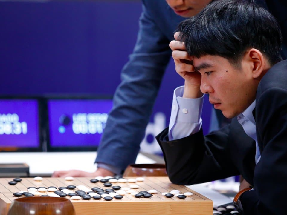
Surprisingly, in March 2016 an algorithm invented by Google DeepMind called Alpha Go defeated Korean world champion in Go 4-1 proving fictional and real-life skeptics wrong. Around a year after that, Alpha Go Zero – the next generation of Alpha Go Lee (the one beating Korean master) – was reported to destroy its predecessor 100-0, being very doubtfully reachable for humans.
Alpha Go/Zero system is a mix of several methods assembled into one great engineering piece of work. The core components of the Alpha Go/Zero are:
- Monte Carlo Tree Search (certain variant with PUCT function for tree traversal)
- Residual Convolutional Neural Networks – policy and value network(s) used for game evaluation and move prior probability estimation
- Reinforcement learning used for training the network(s) via self-plays
In this post we will focus on Monte Carlo Tree Search only.
Introduction
Monte Carlo Tree Search was introduced by Rémi Coulom in 2006 as a building block of Crazy Stone – Go playing engine with an impressive performance.
From a helicopter view Monte Carlo Tree Search has one main purpose: given a game state to choose the most promising next move. Throughout the rest of this post we will try to take a look at the details of Monte Carlo Tree Search to understand what we mean by that. We will also refer back to Alpha Go/Zero from time to time trying to explain what MCTS variant has been used in Deepmind’s AI.
Finite Two Person Zero-Sum Sequential Game
The framework/environment that Monte Carlo Tree Search operates within is a game which by itself is a very abstract broad term, therefore here we focus on a single game type*: Finite Two Person Zero-Sum Sequential Game – which sounds complex at first but it is in fact pretty simple, let’s break it down to the bits:
- game means we deal with an interactive situation. There is interaction between some actors involved (one or more)
- a word finite indicates there is a finite ways of interacting between actors in any point in time
- two person finite game implies two actors being involved in our game
- sequential because players make their moves in sequence – one after another
- and finally, zero-sum game – means the two parties involved have the opposite goal, in other words: in any terminal state of the game the sum of gains for all players equals zero. Sometimes such a game is also called strictly competitive
One can easily verify that Go, Chess or Tic-Tac-Toe are finite two person zero-sum sequential games. Indeed, there are two players involved, there is always finite amount of moves a person may perform and the game is strictly competitive – the goals of both players are completely opposite (all games’ outcomes sum up to zero)
*Please be aware that for the sake of simplicity of this tutorial we focus on certain subset of possible scenarios, Monte Carlo Tree Search is a much broader tool and is applicable outside of finite two person zero-sum games. Go to Monte Carlo Tree Search survey for comprehensive overview.
How to represent a game?
Formally (check this free book for a game theory overview), a game is represented by a bunch of basic mathematical entities. In a PhD level game theory book you may find the following definition:
\[\Gamma_{E} = \{\mathcal{X}, \mathcal{A}, I, p, \alpha, \mathcal{H}, H, \iota, \rho, u\}\]which is very hairy already, diving deep there equals lots of fun for a mathematician, maybe.
From a computer programmer point of view a formal definition might be a bit confusing and possibly hard to work with. Fortunately though we can use a well-known data structure to represent a game in a simplified form: a game tree.
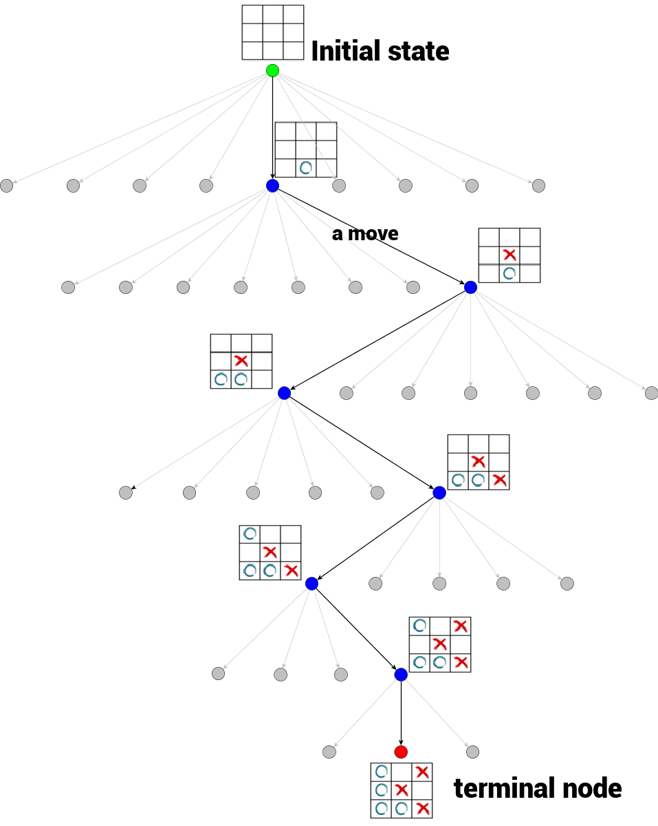
A game tree is a tree in which every node represents certain state of the game. Transition from a node to one of its children (if they exist) is a move. The number of node’s children is called a branching factor. Root node of the tree represents the initial state of the game. We also distinguish terminal nodes of the game tree – nodes with no children, from where game cannot be continued anymore. The terminal node’s states can be evaluated – this is where game result is concluded.
Let’s try to describe the tic-tac-toe game tree you (partially) see:
- at the very top, you can see the root of the tree, representing the initial state of the tic-tac-toe game, empty board (marked green)
- any transition from one node to another represents a move
- branching factor of tic-tac-toe varies – it depends on tree depth
- game ends in a terminal node (marked red)
- the tree traversal from the root to the terminal node represents a single game playout
To limit a game tree size, only visited states are expanded, unexpanded nodes are marked gray.
Game tree is a recursive data structure, therefore after choosing the best move you end up in a child node which is in fact a root node for its subtree. Therefore you can think of a game as a sequence of “the most promising next move” problems represented by a game tree every time (with different root node). Very often in practice, you do not have to remember the path leading to your current state, as it is not a concern in a current game state.
What is the most promising next move? Very shortly about minimax and alpha-beta pruning
Once again, our ultimate goal is to find the most promising next move assuming given game state and the game tree implied. But what would that actually mean?
There is no straight answer to this. First of all, you do not know your opponent’s strategy in advance – he/she may play the perfect game or may be far from a good player. Let’s assume Chess. Knowing that your opponent is an amateur (mathematician would say “knowing your opponent mixed strategy”) you may choose simple strategy to try trick him and win quickly. But the same strategy against a strong opponent would turn against you. That’s obvious.
If you don’t know your opponent at all there is one very radical strategy called minimax that maximizes your payoff assuming your opponent plays the best possible game. In two person finite zero-sum sequential game between A and B (where A maximizes his utility and B tries to minimize it), the minimax algorithm may be described by the following recursive formula:
\[\begin{align} v_A(s_i) &= \max_{a_i} v_B(\text{move}(s_i, a_i)) \quad \text{with} \quad v_A(\hat{s}) = \text{eval}(\hat{s}) \\ v_B(s_i) &= \min_{a_i} v_A(\text{move}(s_i, a_i)) \quad \text{with} \quad v_B(\hat{s}) = -\text{eval}(\hat{s}) \end{align}\]where
- \( v_A \) and \( v_B \) are utility functions for players A and B respectively (utility = gain, payoff)
- \( \text{move} \) is a function that produces the next game state (one of the current node’s children) given current state \( s_i \) and action at that state \( a_i \)
- \( \text{eval} \) is a function that evaluates the final game state (at terminal node)
- and \( \hat{s} \) is any final game state (a terminal node)
- minus sign at \( v_B \) for terminal state is to indicate that game is a zero-sum game – no need to worry!
Simply speaking, given state \( s \) you want to find a move \( a_i \) that will result in the biggest reward assuming your opponent tries to minimize your reward (maximize his). Hence the name minimax. This sounds almost good. All we need is to expand the whole game tree and backpropagate the value with respect to rules given by our recursive formula.
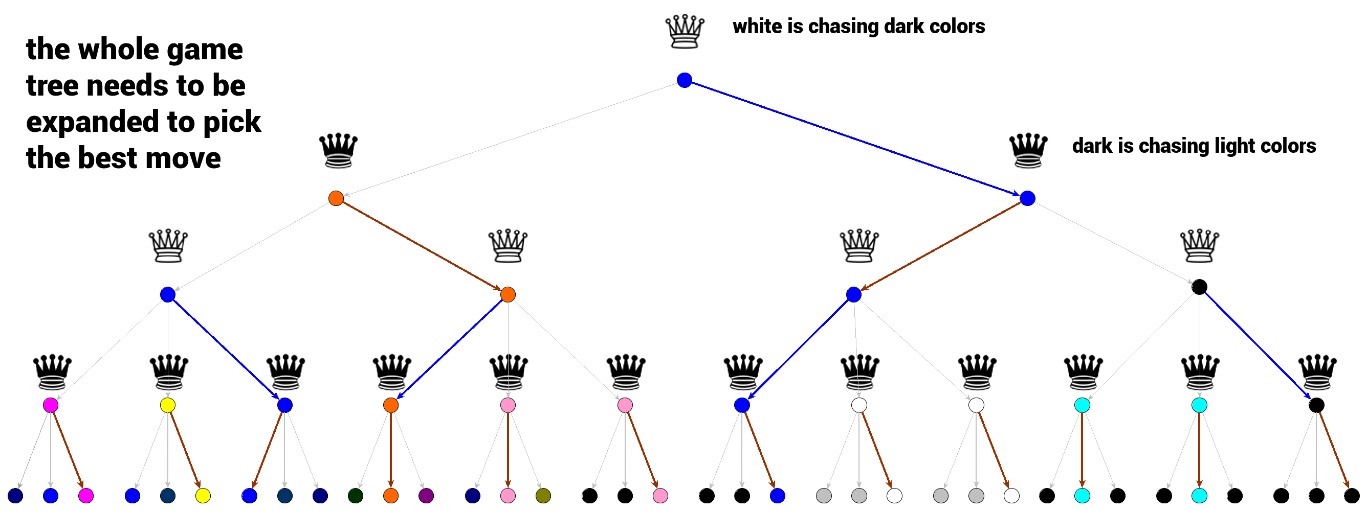
The game tree above illustrates the choice of the best move in minimax algorithm. The white queen wants the game result to be as dark (cold) as possible (reward = pixel intensity) while dark queen will follow the paths leading to the lightest (warmest) colors. Every choice on every level is optimal in minimax sense. We can start from the bottom terminal nodes where the choice is obvious. Dark queen will always pick the lightest color. Then the white queen will chase her maximal reward and choose the path leading to the darkest color. And so on… up to the node representing the current game state. This is how basic minimax algorithm works.
The biggest weakness of minimax algorithm is the necessity to expand the whole game tree. For games with high branching factor (like Go or Chess) it leads to enormous game trees and so certain failure.
Is there a remedy for this?
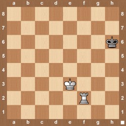
There are a few. One way to go is to expand our game tree only up to certain threshold depth ( d ). But then we are not guaranteed that any node at our threshold tree level ( d ) is terminal. Therefore we need a function that evaluates a non-terminal game state. This is very natural for humans: by looking at Chess or Go board you may be able to predict the winner even though the game still continues. For example, it is rather formality to end the game below:
Another way to overcome game tree size problem is to prune the game tree via alpha-beta pruning algorithm. Alpha-beta pruning is boosted minimax. It traverses the game tree in minimax-fashion avoiding expansion of some tree branches. The result is at best the same as minimax – alpha-beta pruning guarantees improvement by reduction of the search space, though.
The intuitive introduction to minimax and alpha-beta pruning can be found here. Minimax/Alpha-beta pruning is already a very mature solution and is being used in various successful game engines nowadays like Stockfish – the main rival of Alpha Zero in a set of games played at the end of 2017 in somewhat controversial tone.
Monte Carlo Tree Search – basic concepts
In Monte Carlo Tree Search algorithm – the scope of our post today – the most promising move is computed in a slightly different fashion. As the name suggests (especially its Monte Carlo component) – Monte Carlo Tree Search simulates the games many times and tries to predict the most promising move based on the simulation results.
The main concept of Monte Carlo Tree Search is a search. Search is a set of traversals down the game tree. Single traversal is a path from a root node (current game state) to a node that is not fully expanded. Node being not fully expanded means at least one of its children is unvisited, not explored. Once a not fully expanded node is encountered, one of its unvisited children is chosen to become a root node for a single playout/simulation. The result of the simulation is then propagated back up to the current tree root updating game tree nodes’ statistics. Once the search (constrained by time or computational power) terminates, the move is chosen based on the gathered statistics.
Lots of dots not clearly connected together, right?
Let’s try to ask crucial questions regarding the simplified description above to slowly understand all the pieces:
- What are expanded or not fully expanded game tree nodes?
- What does it mean “to traverse down” during search? How is the next (child) node selected?
- What is a simulation?
- What is the backpropagation?
- What statistics are back-propagated and updated in expanded game tree nodes?
- How is the final move even chosen?
Again, stay focused, we will get there soon, bit by bit.
Simulation/Playout
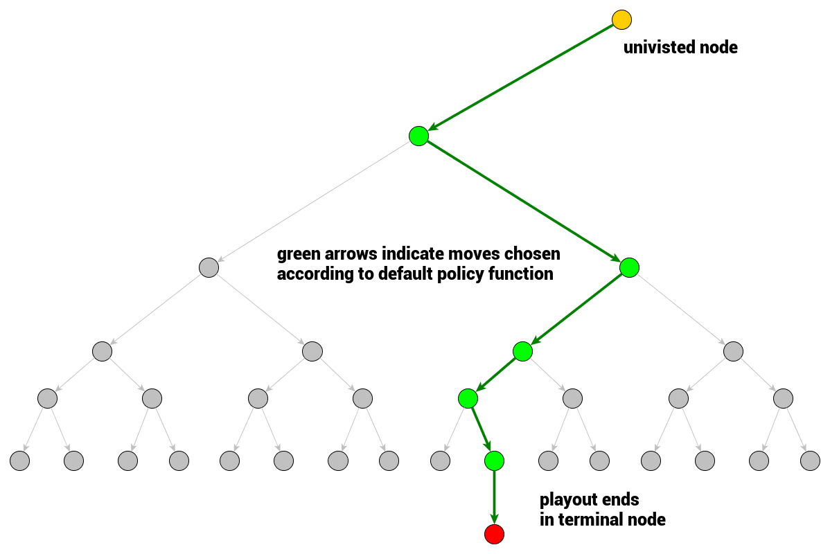
Let’s focus on simulation (or playout equivalently) first as it does not rely on other terms’ definitions heavily. Playout/simulation is a single act of a game play – a sequence of moves that starts in current node (representing game state) and ends in a terminal node where game result can be computed. Simulation is a game tree node evaluation approximation computed by running a somehow random game starting at that node.
How are the moves chosen during simulation?
During simulation the moves are chosen with respect to a function called rollout policy function:
\[\text{RolloutPolicy}: s_i \rightarrow a_i\]that consumes a game state and produces the next move/action. In practice, it is designed to be fast to allow many simulations being played quickly – default rollout policy function is a uniform random.
Playout/Simulation in Alpha Go and Alpha Zero
In Alpha Go Lee evaluation of the leaf \( S_L \) is a weighted sum of two components:
\[V(S_L) = (1 - \alpha) \, v_0(S_L) + \alpha \, z_L\]
- standard rollout evaluation \( z_L \) with custom fast rollout policy that is a shallow softmax neural network with handcrafted features
- position evaluation given by 13-layer convolutional neural network \( v_0 \) called Value Network trained on 30 million of distinct (no two positions come from the same game) positions extracted from Alpha Go self-plays
In Alpha Zero DeepMind’s engineers went a step further, they do not perform playouts at all, but directly evaluate the current node with a 19-layer CNN Residual neural network (in Alpha Zero they have one network \( f_0 \) that outputs position evaluation and moves probability vector at once)
\[V(S_L) = f_0(S_L)\]
Simulation/rollout in a simplest form is then just a random sequence of moves that starts at given game state and terminates. Simulation always results in an evaluation – for the games we talked about it is a win, loss, or a draw, but generally any value is a legitimate result of a simulation.
In Monte Carlo Tree Search, simulation always starts at the node that has not been visited previously – we will learn what a visited node means in a minute.
Game tree node expansion – fully expanded and visited nodes
Let’s think about how humans think about games such as Go or Chess.
Given a root node plus the rules of the game the rest of the game tree is already implied. It pops up and we can traverse it without storing the whole tree in the memory. In its initial form though it is not expanded at all. In the very initial game state we are at the root of the game tree and the remaining nodes are unvisited. Once we consider a move, we imagine a position a move would result in. Somehow we visit a node analyzing (evaluating) the position a move would bring. Game states that you never even considered visiting remain unvisited and their potential is undiscovered.
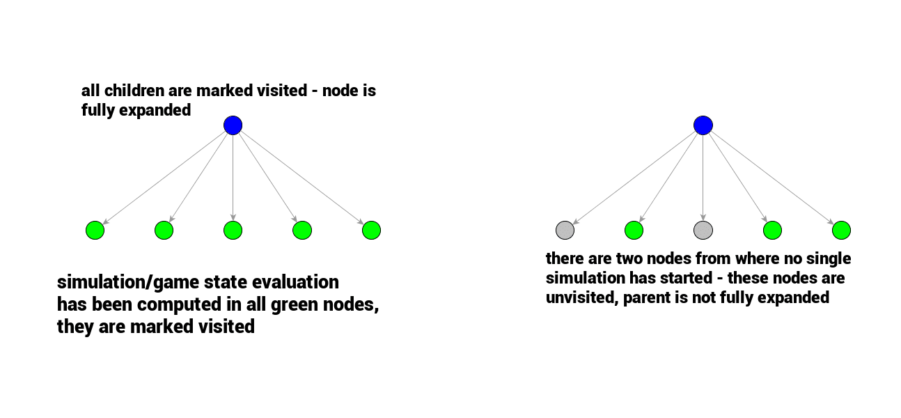
The same distinction applies to Monte Carlo Tree Search game tree. Nodes are considered visited or unvisited. What does it mean for a node to be visited? Node is considered visited if a playout has been started in that node – meaning it has been evaluated at least once. If all children nodes of a node are visited, the node is considered fully expanded, otherwise – well – it is not fully expanded and further expansion is possible.
In practice then, at the very beginning of a search all of the root node’s children are unvisited – one is picked and first simulation (evaluation) starts right away.
Please be aware that nodes chosen by rollout policy function during simulation are not considered visited. They remain unvisited even though a rollout passes through them, only the node where simulation starts is marked visited.
Backpropagation – propagating back the simulation result
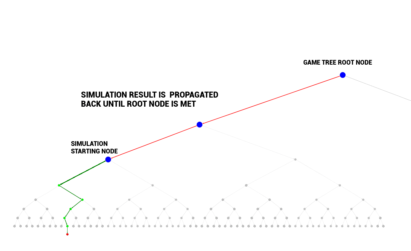
Once simulation for a freshly visited node (sometimes called a leaf) is finished, its result is ready to be propagated back up to the current game tree root node. The node where simulation started is marked visited.
Backpropagation is a traversal back from the leaf node (where simulation started) up to the root node. Simulation result is carried up to the root node and for every node on the backpropagation path certain statistics are computed/updated. Backpropagation guarantees that every node’s statistics will reflect results of simulations started in all its descendants (as the simulation results are carried up to the game tree root node).
Nodes’ statistics
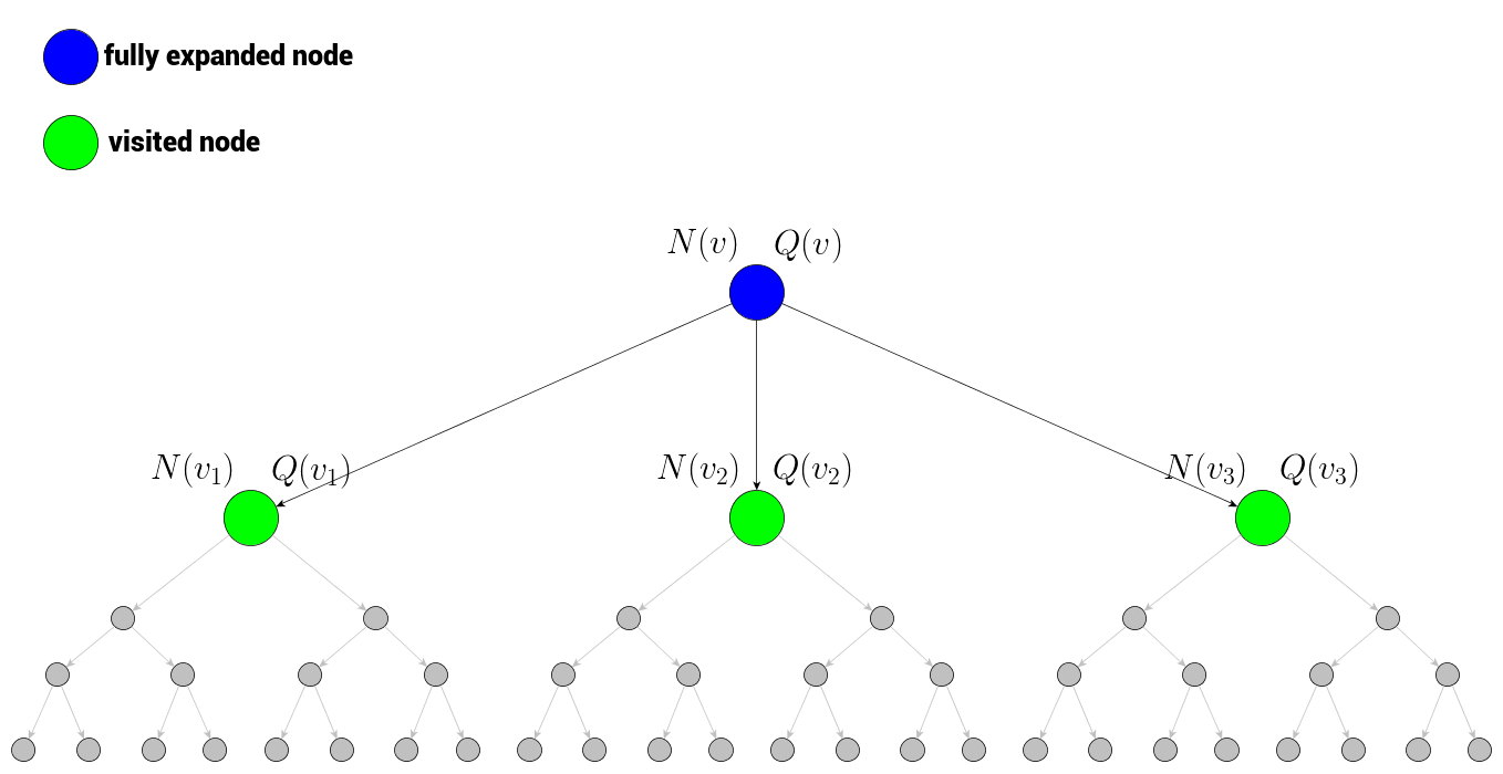
The motivation for back-propagating simulation result is to update the total simulation reward \( Q(v) \) and total number of visits \( N(v) \) for all nodes \( v \) on backpropagation path (including the node where the simulation started).
- \( Q(v) \) – Total simulation reward is an attribute of a node \( v \) and in a simplest form is a sum of simulation results that passed through the considered node.
- \( N(v) \) – Total number of visits is another attribute of a node \( v \) representing a counter of how many times a node has been on the backpropagation path (and so how many times it contributed to the total simulation reward)
These two values are maintained for every visited node; once a certain number of simulations is finished, visited nodes will store information indicating how exploited/explored they are.
In other words, if you look at a random node’s statistics these two values will reflect how promising the node is (total simulation reward) and how intensively explored it has been (number of visits). Nodes with high reward are good candidates to follow (exploitation), but those with low amount of visits may be interesting too (because they are not explored well).
One puzzle is still missing. How do we get from a root node to the unvisited node to start a simulation?
Game tree traversal
Well, at the very beginning of the search, since we have not started any simulations yet, unvisited nodes are chosen first. Single simulation starts at each of them, results are backpropagated to the root node and then root is considered fully expanded.
But what do we do next? How do we now navigate from a fully expanded node to an unvisited node? We have to go through the layers of visited nodes and so far there is no recipe how to proceed.
To pick the next node on our path to starting the next simulation via fully expanded node \( v \) we need to consider information about all children of \( v \): \( v_1, v_2, \dots, v_k \) and the information about the node \( v \) itself. Let’s think about what information is available now:
Our current node – marked blue – is fully expanded so it must have been visited and so stores its node statistics: total simulation reward and total number of visits. The same applies to its children. These values are components of our last piece: Upper Confidence Bound applied to trees or shortly UCT.
Upper Confidence Bound applied to trees
UCT is a function that lets us choose the next node among visited nodes to traverse through – the core function of Monte Carlo Tree Search:
\[\operatorname{UCT}(v_i, v) = \frac{Q(v_i)}{N(v_i)} + c \sqrt{\frac{\ln N(v)}{N(v_i)}}\]Node maximizing UCT is the one to follow during Monte Carlo Tree Search tree traversal. Let’s see what the UCT function does:
First of all, our function is defined for a child node \( v_i \) of a node \( v \). It is a sum of two components – the first component of our function \( \frac{Q(v_i)}{N(v_i)} \), also called exploitation component, can be read as a winning/losing rate – we have total simulation reward divided by total number of visits which estimates win ratio in the node \( v_i \). This already looks promising – at the end of the day we might want to traverse through the nodes that have high winning rate.
Why can’t we use exploitation component only? Because we would very quickly end up greedily exploring only those nodes that bring a single winning playout very early at the beginning of the search.
Quick example:
Let’s assume we start Monte Carlo Tree Search routine using exploitation UCT component only. Starting from a root node we run a simulation for all children and then in the next steps only visit those for which simulation result is at least one win. Nodes for which first simulation was unlucky (please recall default policy function that is very often random in practice) would be abandoned right away without any chance to improve.
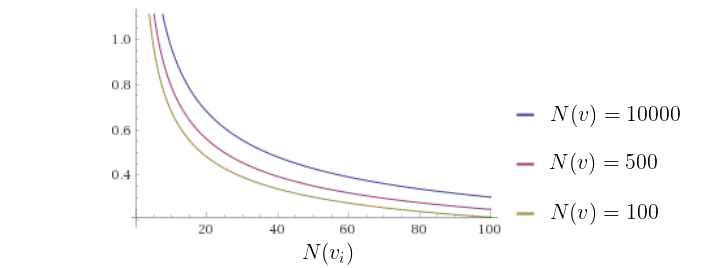
Therefore we have a second component of UCT called exploration component. Exploration component favors nodes that have not been explored – those that have been relatively rarely visited (those for which \( N(v_i) \) is lower). Let’s take a look at the shape of exploration component of UCT function – it decreases with numbers of visits in a node and will give high chance of selection for less-visited nodes directing the search towards exploration.
Finally, parameter \( c \) in the UCT formula controls the trade-off between exploitation and exploration in Monte Carlo Tree Search.
UCT in Alpha Go and Alpha Zero
In both Alpha Go Lee and Alpha Zero the tree traversal follows the nodes that maximize the following UCT variant:
\[\operatorname{UCT}(v_i, v) = \frac{Q(v_i)}{N(v_i)} + c \, P(v, v_i) \frac{\sqrt{N(v)}}{1 + N(v_i)}\]where \( P(v, v_i) \) is prior probability of the move (transition from \( v \) to \( v_i \) ), its value comes from the output of deep neural network called Policy Network. Policy Network is a function that consumes game state and produces probability distribution over possible moves (please note this one is different from fast rollout policy). The purpose here is to reduce the search space to the moves that are reasonable – adding it to exploration component directs exploration towards the reasonable moves.
Policy network training in Alpha Go and Alpha Zero
There are two policy networks in Alpha Go:
- SL Policy Network that is trained in a supervised fashion based on human games dataset.
- RL Policy Network – boosted SL Policy Network – it has the same architecture but is further trained via Reinforcement Learning (self-plays)
Interestingly – in DeepMind’s Monte Carlo Tree Search variant – SL Policy Network output is chosen for prior move probability estimation \( P(v, v_i) \) as it performs better in practice (authors suggest that human-based data is richer in exploratory moves). What is the purpose of the RL Policy Network then? The stronger RL Policy Network is used to generate 30 million positions dataset for Value Network training (the one used for game state evaluation).
In Alpha Zero on the other hand there is only one network \( f_0 \) that is both Value and Policy Network. It is trained entirely via self-play starting from random initialization. There is a number of networks trained in parallel and the best one is chosen for training data generation every checkpoint after evaluation against best current neural network.
One important remark on UCT function: in competitive games its exploitation component \( Q_i \) is always computed relative to the player who moves at node \( i \) – it means that while traversing the game tree perspective changes depending on a node being traversed through: for any two consecutive nodes this perspective is opposite.
Terminating Monte Carlo Tree Search
We now know almost all the pieces needed to successfully implement Monte Carlo Tree Search, there are few questions we need to answer though. First of all when do we actually end the MCTS procedure? The answer to this one is: it depends on the context. If you build a game engine then your “thinking time” is probably limited, plus your computational capacity has its boundaries, too. Therefore the safest bet is to run MCTS routine as long as your resources let you.
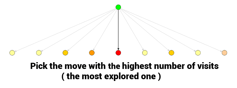
Once the MCTS routine is finished, the best move is usually the one with the highest number of visits \( N(v_i) \) since its value has been estimated best (the value estimation itself must have been high as it’s been explored most often, too).
After picking your move using Monte Carlo Tree Search, your node of choice will become a game state for your opponent to move from. Once he picks his move – again – you will start Monte Carlo Tree Search routine starting from a node representing a game state chosen by your opponent. Some statistics from previous MCTS rounds may still be in that new branch you are now considering. This brings an idea of reusing the statistics instead of building new tree from scratch – and in fact this is what creators of Alpha Go / Alpha Zero did, too.
Monte Carlo Tree Search – summary
Having all the bits together, let’s try to recall the very first simplified description of Monte Carlo Tree Search and enclose it in pseudo-code:
1
2
3
4
5
6
7
8
9
10
11
12
13
14
15
16
17
18
19
20
21
22
23
24
25
26
27
28
29
30
def monte_carlo_tree_search(root):
    while resources_left(time, computational_power):
        leaf = traverse(root)  # leaf = unvisited node
        simulation_result = rollout(leaf)
        backpropagate(leaf, simulation_result)
    return best_child(root)

def traverse(node):
    while fully_expanded(node):
        node = best_uct(node)
    return pick_unvisited(node.children) or node  # in case no children are present or node is terminal

def rollout(node):
    while not is_terminal(node):
        node = rollout_policy(node)
    return result(node)

def rollout_policy(node):
    return pick_random(node.children)

def backpropagate(node, result):
    if node is None:
        return
    node.visits += 1
    node.total_reward += result
    backpropagate(node.parent, result)

def best_child(node):
    # pick child with highest number of visits
    return max(node.children, key=lambda c: c.visits)
As you can see, it reduces to very few set of functions that could work for any game of your choice, not only Go or Chess.
Example implementations
That would be all folks, I hope you enjoyed the read and the content here helped you understand Monte Carlo Tree Search – writing it definitely helped me wrap my head around it.
The very next step (hopefully material for the next post) is trying to implement a simple chess bot with components similar to AlphaGo: Value and Policy Network plus MCTS (some work on that – still in progress though – can be found here) Please check out Leela Chess Zero for further inspiration!
