Attention mechanism in NLP – beginners guide
The field of machine learning is changing extremely fast for last couple of years. Growing amount of tools and libraries, fully-fledged academia education offer, MOOC, great market demand, but also sort of sacred, magical nature of the field itself (calling it Artificial Intelligence is pretty much standard right now) – all these imply enormous motivation and progress. As a result, well-established ML techniques become out-dated rapidly. Indeed, methods known from 10 years ago can often be called classical.
This sort of revolution has happened recently. The default architectural choice for NLP related problems, recurrent neural network, has been seriously challenged – to say the least. This very solid architecture is being quickly replaced by networks based on attention mechanism only that drops RNN entirely achieving at least comparable (and often better) performance both in NLP and Computer Vision.
This post is an attempt to go through the most significant papers related to attention mechanism with the goal to grasp basic knowledge and intuition about it. We will start by looking at its very first NLP application where it was introduced to solve neural machine translation in 2015. Then we will go through improvements to attention introduced in Transformer – neural networks architecture that uses one specific variant of attention mechanism as its main building block – skipping thus far seemingly necessary recurrent connections.
Attention mechanism for neural translation, 2015
Attention that we know today was first proposed for the problem of machine translation in paper titled Neural Machine Translation by Jointly Learning to Align and Translate submitted to ICLR 2015. Its purpose was to enhance “traditional” Encoder-Decoder Recurrent Neural Network based machine translation. Interestingly, in this paper authors don’t even call it “attention” directly – they only use words “attention”, “pay attention” when they try to provide human-friendly interpretation of the mechanism they introduce.
Let’s try to take a closer look at the RNN-based machine translation without attention mechanism first – as it had been a scaffold architecture for attention mechanism introduced next.
Attention-less Neural Machine Translation, RNN Encoder-Decoder
Attention-less neural machine translation that we will present now is an example of sequence to sequence modeling. In these types of problems we get sequence of vectors as input and our task is to produce target sequence of vectors (often with no sequence length constraints on both ends). In case of language translation, we deal with two sequences of vectors: one representing input sequence we want to translate and corresponding sequence representing its translation.
In 2014 Kyunghyun Cho and his colleagues proposed a solution to machine translation problem via neural network called RNN Encoder-Decoder. This work was a foundation of attention mechanism introduced in authors’ next paper.
Let’s take a look at the diagram below depicting RNN Encoder-Decoder neural machine translator architecture.
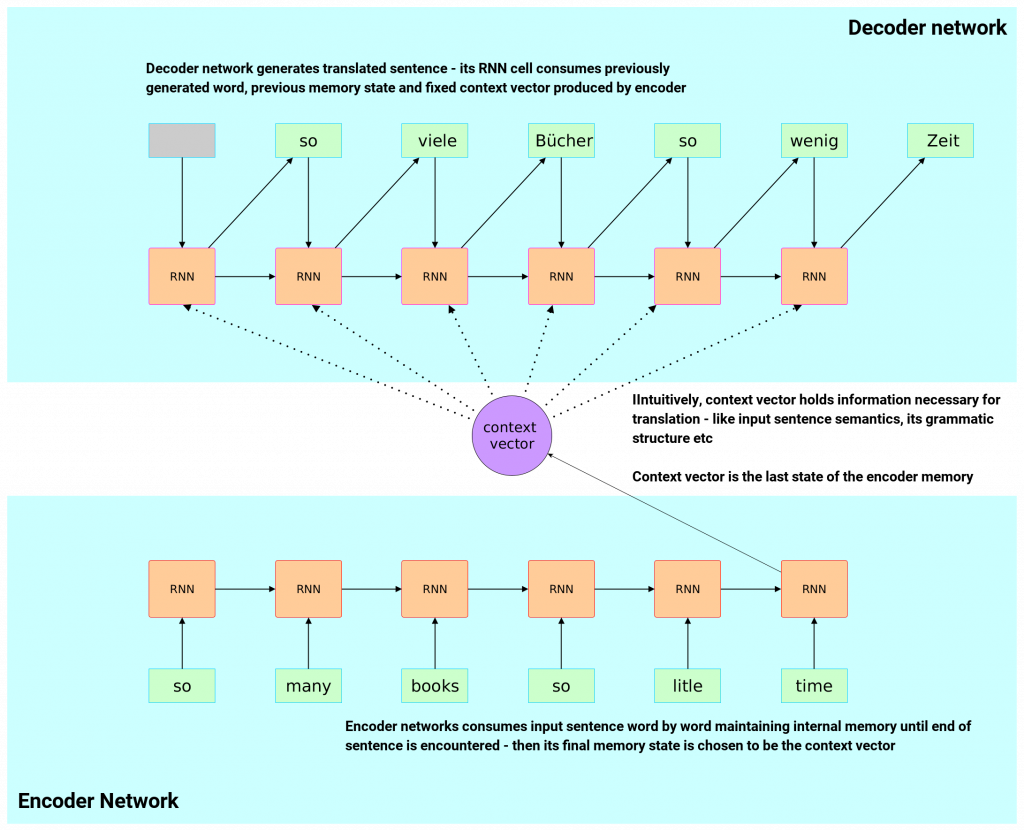
As you can see, the whole neural translator architecture is composed of two Recurrent Neural Networks glued together – one is called Encoder and the other one called Decoder.
Input sentence flows through Encoder network word by word – network gathers information about the sentence in its internal memory. Decoder’s job is to produce proper translation (using information gathered by encoder in the form on context vector – last Encoder hidden memory state).
Details of RNN Encoder-Decoder cells
Let’s take a closer look at the Encoder and Decoder in some details too. Here is the diagrams of Encoder (bottom) and Decoder (top) cells with some thoughts thrown below:
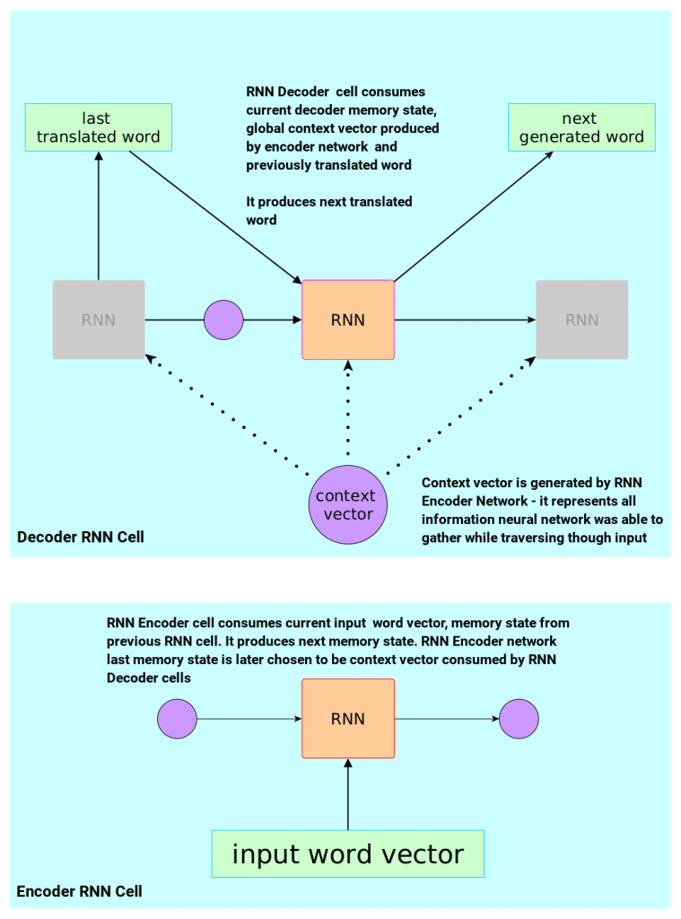
Decoder Cell
Decoder cell is an RNN cell with the following “interface”:
- At the beginning of the translation (when no word is yet generated) it consumes special blank symbol, initial hidden memory state (which often is initialized to be a zero vector) and global context vector – having that information it computes first translated word.
- For consecutive words (once some words are already there) it consumes previously generated word, the same global context vector and current hidden memory state that decoder maintain internally (the intuition here is that hidden memory state will “remember” what information has already been included in the translation, maybe currently generated local grammar construct, semantics etc)
- Translation is finished when special symbol
[EOS](end-of-sentence) is generated - Actual version of RNN is described in this paper (but for simplicity let’s just blackbox it).
Encoder Cell
Encoder cell is a bit simpler as it does not consume any additional context (in fact it’s job is to generate one). Single cell of encoder works as follows:
- At the beginning of the input sentence processing (when no word is yet seen) it consumes first word, initial hidden memory (which we can assume is zero vector) – having that information it computes first internal hidden memory state and “remembers” it)
- For consecutive words (once some words are already seen) it consumes the next word and current hidden memory state
- Input sentence processing is finished when special symbol
[EOS]is seen – then network outputs current hidden memory state – which is also aforementioned global context vector that decoder consumes at each step. - Actual version of RNN is described in this paper (again, let’s blackbox it for simplicity)
RNN Encoder-Decoder Summary
The most important bit to remember here is context vector being fixed throughout the decoding (translating) phase. Decoder consumes the same global context vector for translation generation at each time step. It uses the same information derived from encoder network to generate all translated words.
This type of context representation turned out to be problematic, especially for long sentences (Curse of Sentence Length).
The Curse of Sentence Length was also a motivation for attention mechanism that changed the way context vector was represented. With attention mechanism in place there is no one global context vector anymore but rather specific context for every translated word at every time step – this specific context also represents attention our neural machine translator pays to particular parts of input sentence any time it generates a word.
Neural Machine Translation with Attention
The main problem of RNN Encoder-Decoder architecture for machine translation was its inability to handle long sentences. The intuition here is that global context vector of long sentences is losing some information and so it is not able to capture the whole sentence grammatical structure and its full semantics. First attempt to overcome this issue was to try automatic segmentation but the real – what later turned out to be – huge breakthrough came with attention mechanism introduced in ‘Neural Machine Translation by Jointly Learning to Align and Translate’.
Authors modified RNN Encoder-Decoder network in a way that context vector was no longer fixed – it was not global. To achieve that they proposed changes to both Encoder and Decoder networks.
Changes proposed to Encoder Network
The original purpose of Encoder network for RNN Encoder-Decoder was to figure out one fixed vector representing information that is necessary for translation. This was achieved via unidirectional RNN. Sentence was consumed word by word to produce single fixed context vector.
In attention paper, authors proposed an alternative to single fixed context vector – a weighted sum of annotations. Annotations represented local information about particular words from input sentence.
Upgraded Encoder Network job was to produce that local information about every single word – annotations.
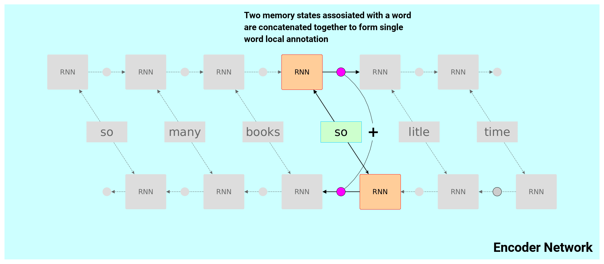
Let’s take a look at that improved Encoder architecture below:
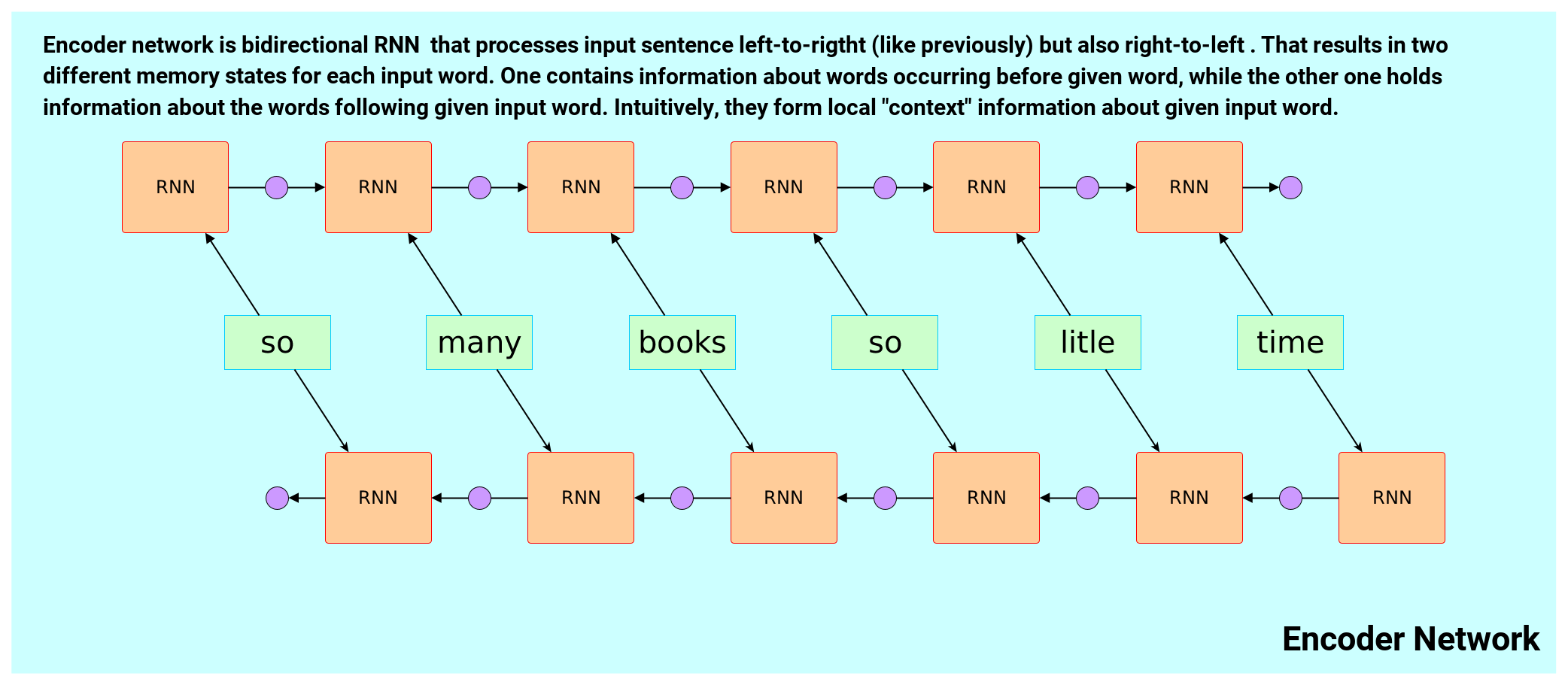
Encoder network is now bi-directional – it will read input sentence from left to right and from right to left producing two hidden RNN memory states for each word. These states are concatenated together composing so called “annotations.”
Annotations are supposed to model local context of each word in an input sentence. You may think of them as vectors of information computed on-the-fly in training phase. The intuition is that these annotations will encode semantics, possibly grammar and in general any magic sauce needed for translation of that particular word.
Decoder network
Decoder network of our upgraded neural translator remains uni-directional RNN. Its main job is to generate translated words. It will maintain its internal state (information seen so far) but also consume specially crafted digest of aforementioned annotations.
Our digest of annotations is given by a weighted sum of all annotations. Let’s black-box weights for simplicity now – we will explain that in a moment.

RNN Decoder network consumes the following components when it tries to figure out the next word:
- Its current internal state $s_{i-1}$ – this vector encodes everything Decoder RNN “saw” up to that point
- Set of annotations $ {h_1, … h_{T_x}} $ – one for each input word – that are magically combined into $ c_i $
Attention mechanism
The way set of annotations from input sentence is combined together into one dynamic local context vector is actually closely related to mechanism we are after – attention.
In paper of our interest here authors used weighted combination of annotations in a following way:
-
Single scalar weight is computed for each annotation vector via the formula:
\[\alpha_j= \frac{\exp(e_j)}{\sum_{i =1}^{T_x} \exp(e_i)}\]
which is a softmax over some “energy” vector.
- Each component of an energy vector is modeled via:
where FFN is feed forward shallow neural network.
It is important to note that our FNN models how much attention RNN Decoder should pay to input annotations. Another important observation is that FNN consumes “current” decoder RNN state $ s_{i-1} $ and single word annotation $ h_i $.
One interpretation that we will find useful in a moment is to consider the decoder current state to be a query seeking for importance of annotations in current translation moment with FNN being a logic providing the way of computing this importance.
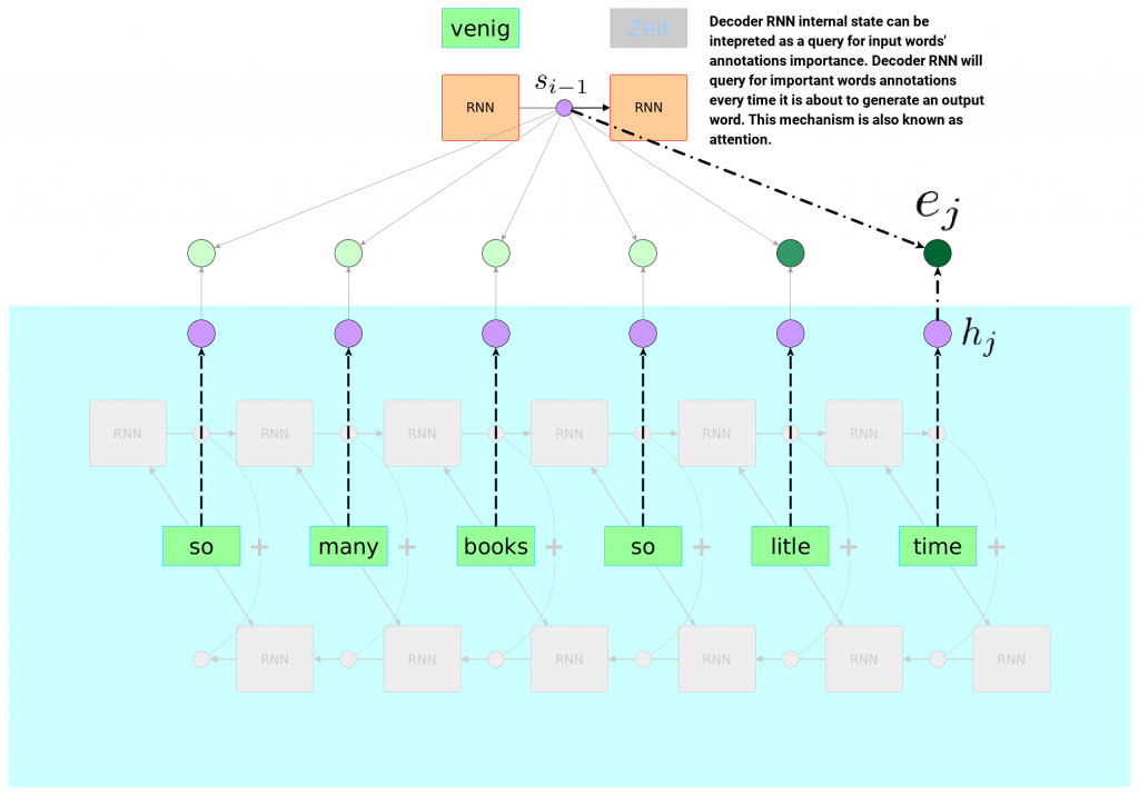
At the moment when new target translated word is about to be generated, Decoder RNN may “know” (by its hidden state) that the next word is – for example – a physical object – it may also know some of its properties like sittable, made-of-wood. It then can “query” annotations with that information via FNN. As a result of such query bunch of energy values is returned – one for each annotation – that are later squashed via softmax to compose our final weighted sum, which is then an input to RNN cell producing the next word. You can imagine that FNN would return very high value for energy corresponding to the input word “chair”.
Self attention and other follow up ideas
After its first success in neural translation domain, attention mechanism slowly kicked in. People started to build on top of it – simplifying or extending original formulation. Starting from 2015 until 2017, the common theme was to train bi-directional encoder to get annotations that decoder could attend through attention mechanism. Broad range of different interesting ideas started to emerge – like self-attention in Long Short-Term Memory-Networks for Machine Reading where authors proposed extension to LSTM to include attention mechanism. Attention was present in A Deep Reinforced Model For Abstractive Summarization with successful application to text summarization – generating short text summaries of long texts. In A Structured Self-Attentive Sentence Embedding authors proposed generic attention-based encoder architecture that was a backbone for various NLP tasks (sadly without transfer learning capabilities).
The big breakthrough came in 2017 with paper funnily titled Attention is All You Need where authors proposed architecture called Transformer that was built on top of attention only – with no recurrent neural networks present. Authors also proposed a bit more general view on attention – modelling it in terms of Queries, Keys and Values. Finally, they introduced new variants of attentions – scaled dot-product attention, and multihead-attention built on top of that.
Transformer
Attention mechanism as a function of queries, keys and values
Let’s stay in translation context, in our safe RNN framework and try to revisit attention we already saw. We are going to freeze time in one single moment of translation and try to name all entities involved a bit differently. We no longer want to see annotations and hidden states, but rather Values, Queries and Keys. Let’s see how it would look like:
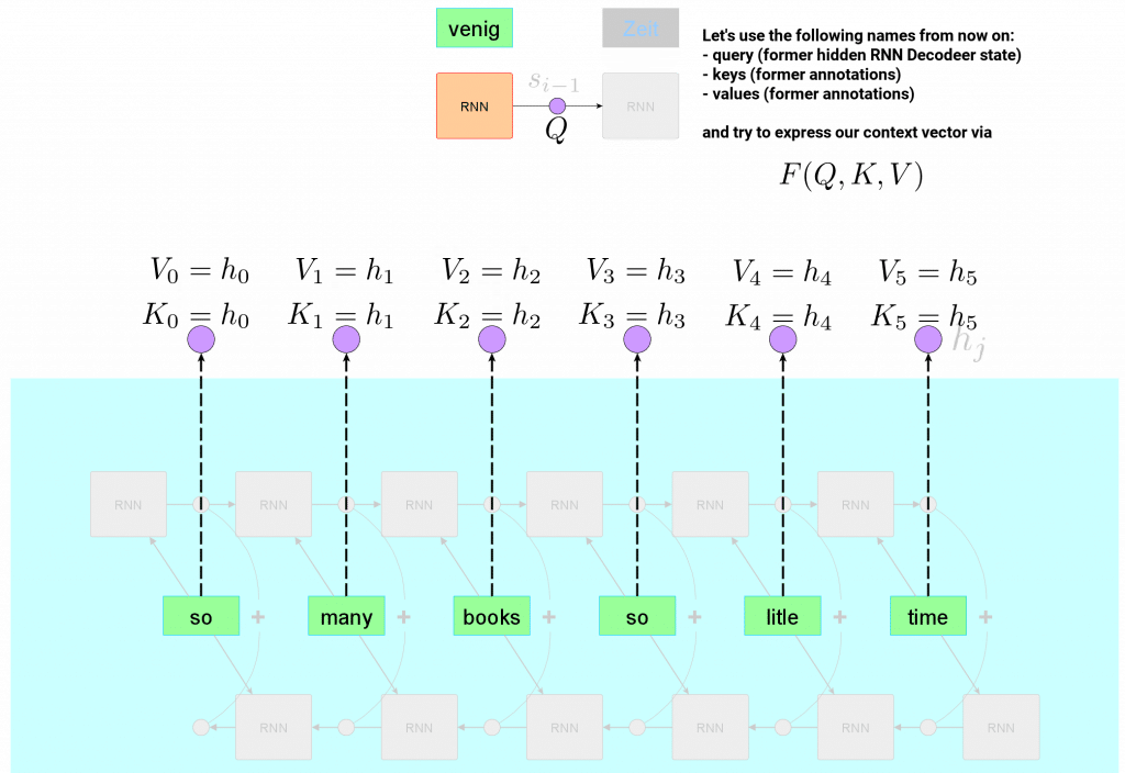
Now attention in our RNN neural translation setup is expressed by:
\[F(Q,K,V) = \text{Softmax}(\text{FNN}(Q, K)) \cdot V\]- $\text{Softmax}(\text{FNN}(Q, K))$ can be understood as compatibility function between given Query and set of Keys
- The result from that compatibility function are weights used for weighted combination of corresponding Values.
Coming back to our translation RNN example, our Query $ Q $ is still hidden state of Decoder network that holds information about current translation state: semantics, grammar etc. Keys and Values are both annotations. We check compatibility of our query with keys via soft-maxed feed forward NN – this gives us “soft” indices of important annotations (Values). Then we return weighed sum of these values – this produces context that is later fed to next RNN cell that will finally produce the next translated word.
In other words:
Attention mechanism
An attention function can be described as mapping a query and a set of key-value pairs to an output, where the query, keys, values, and output are all vectors. The output is computed as a weighted sum of the values, where the weight assigned to each value is computed by a compatibility function of the query with the corresponding key.
“Attention Is All You Need” paper
which comes from original Transformer paper: Attention is All You Need.
Changes to attention
Before we make the major step of dropping RNN let’s still live in our complex – but safe – recurrent neural network world and focus on attention mechanism only.
In Transformer paper the new mechanism of attention was introduced – it was called Multi-Head Scaled Dot-Product Attention. It sounds very involved but it will turn out to be easy in a moment. First of all let’s dismantle it into two parts:
- Scaled Dot-Product Attention
- Multi-Head Attention
Scaled Dot-Product Attention
Scaled Dot-Product Attention can easily be expressed within our generalized framework in terms of Queries, Keys, and Values. The formula changes only slightly. Softmax is kept to produce weights that sum up to 1 but there is no Feed Forward Neural Network involved anymore. The formula of Scaled-Dot-Product Attention is given by:
\[\text{Attention}(Q,K,V) =\text{Softmax}\left(\frac{Q\cdot K^{T}}{\sqrt{d_k}}\right) \cdot V\]The only difference is in what we already called compatibility function – function producing weights for weighted sum of Values. Softmax is kept, but we replace a bit complex FNN with very simple scaled dot-product (hence the name). Here – the intuition is to consider dot-product as a certain measure of similarity between two vectors involved. It is also not very far from being just objective truth – if two vectors involved are normalized, dot-product turns into cosine similarity – heavily present in NLP.
We can loosely interpret Scaled-Dot Product attention as mechanism that would aim attending similar vectors (w.r.t to dot-product).
The scaling factor that we see here – dimensionality of a key vector – is a technical detail that authors figured out empirically – they noticed that without any scaling, softmaxed dot-product could land in high values regions where gradients are small. Scaling it is an attempt to overcome this issue.
To get a bit more familiar with that new type of attention let’s try to picture how it would look like if we used it in our good old recurrent neural network setup (here we happily assume hidden state and annotations are of same dimensionality – to make dot-product possible).
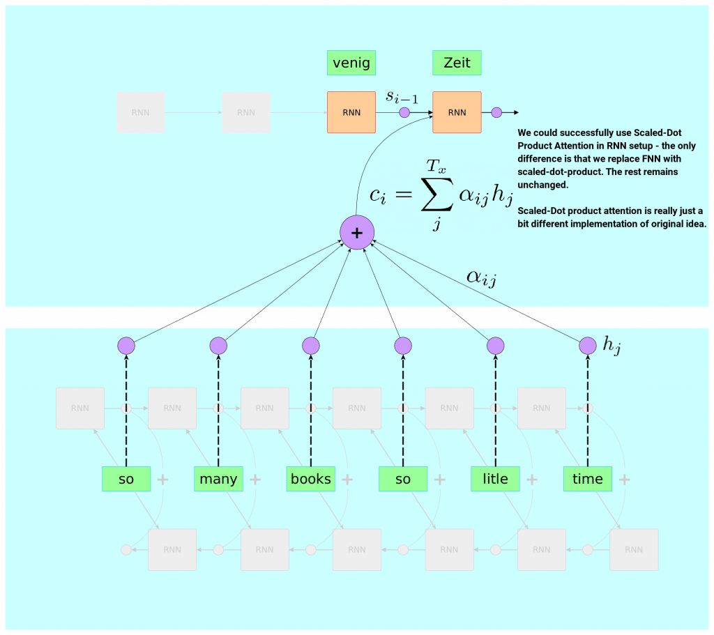
As you can see this is still a tiny detail. Part of compatibility function is replaced by scaled dot-product. The rest remains unchanged. Meaning, that if we felt lucky we could as well try to use Scaled-Dot Product Attention instead of FNN in attention formulation of our RNN-based neural translation model from 2015.
Single-head attention
Before we introduce another improvement to attention mechanism present in Transformer architecture – let’s enclose our Key, Value, Query setup above into single term: Single Head Attention. Simplified version of single head attention is sketched below
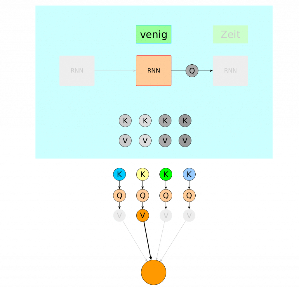
Again, Query is crunched together with bunch of Keys to produce weighted sum of Values as a result – let’s call this setup Single Head Attention so we can smoothly transit into Multi-Head Attention world.
Multi-head attention
Multi-head attention is further generalization of attention.
Attention we know so far – produces weighted sum of Values. Each value is a single vector and so final result is a single vector. To arrive at multi-head attention definition let’s first call this one final vector a head. Using this terminology “normal” attention would always yield one head only. In multi-head attention though we want to deal with N vectors like that – or N heads to later crunch them together into one output.
First, let’s figure out how to arrive to N different heads from one set of query, keys and values.
To get multiple N different heads authors of Transformer added N sets of extra 3 trainable projection matrices (aka dense linear layers) on top of query, keys and values. Single head now looks like:
\[\text{head}_{i} = \text{Attention}(QW_{i}^{Q}, KW_{i}^{K}, VW_{i}^{V})\]This is Scaled Dot-Product attention that we know already but it is applied to projected versions of query, keys and values. Matrices $ W_{i}^{K} $, $ W_{i}^{Q} $, $ W_{i}^{V} $ are our three different projections matrices.
Long story short, one head of multi-head attention is produced by
- First projecting query, keys, values N times via N sets of projection matrices $ W_{i}^{K} $, $ W_{i}^{Q} $, $ W_{i}^{V} $ (one for each head)
- Then crunching these projected versions of query, keys and values through Scaled Dot-Product Attention
Multi-head attention is hyper-parametrized by number of heads – it is up to user how many heads to use. Let’s address final question now: how to combine multiple heads into one final result?
The final output of multi-head attention is produced by:
– Concatenating heads into one vector
– Projecting concatenated heads via another projection matrix $ W_O $
Let’s still keep one leg on a familiar RNN territory and imagine how multi-head attention would like in imaginary neural translation model:
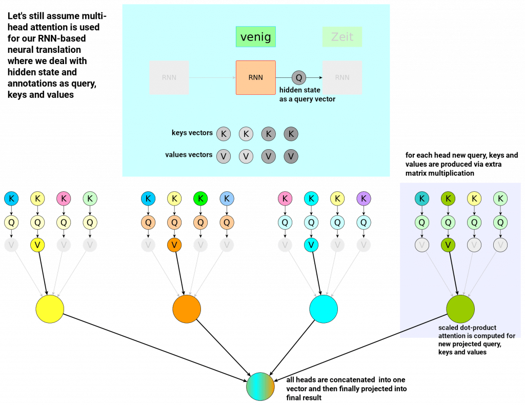
Multi-head attention introduces extra trainable parameters: 3 matrices for each head and one extra matrix for the concatenation. This yields extra expressiveness. In practice it is not that obvious but let’s risk the following statement: Single head may be interpreted as entity modelling single characteristics of the input sentence – you can imagine separate head responsible for understanding semantics, separate head for grammar structure etc.
Simplification by dropping recurrent connections
So far we always assumed queries, keys and values all come from decoder (its hidden state as a query) or encoder (its annotations as keys and values) – both being RNNs. Now we are going to drop this assumption and consider Queries, Keys and Values to be word-embeddings. Let’s see where it leads us.
Quick reminder, word embeddings like word2vec are vectors that are capable of representing words in N-dimensional vector space where often algebraic operations have semantic implications (you can look at some more examples of that phenomenon here). Word-embeddings are good representations of single words – by themselves they don’t encode any information about the context in a particular sentence – they are rather fixed, hardcoded for every single word.
Having word embeddings – like word2vec – in our toolbox we can now consider getting rid of annotations and hidden RNN state and replace them all with embeddings. Of course, at that point we lose some information, the whole idea of annotations being generated by bi-directional encoder was to include some contextual information from given sentence. In word-embedding setup we temporarily lose it.
Let’s consider our input sentence as usual, but this time we:
- Treat word-embedding corresponding to word ‘little’ as a Query:
- Treat all word-embeddings from our input sentence as Keys and Values
- Apply Multi-Head Scaled Dot-Product Attention on top
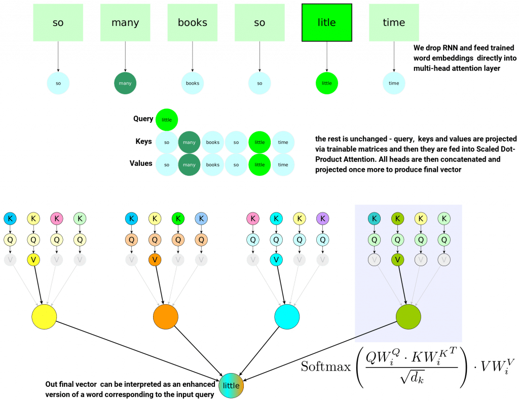
The crucial observation here is that our final vector – result of multi-head attention – can be considered as an enhanced version of a Query – which happens to be a single word. So now our word will contain information about surrounding words in a sentence – because it was crunched with them together via many heads and then projected into final vector. Multi-Head Scaled-Dot Product Attention can therefore be loosely interpreted as enriching word-embeddings with contextual information from a sentence it comes from. We can even enforce same dimensionality easily because this is just a matter of final projection matrix size. We can choose it to match original input size and so input and output would have same size.
In that setup – where we choose projection matrix sizes to yield same input output dimensionality, we can actually think about Multi-Head Scaled-Dot Product Attention as a parametrized function that consumes a word and sentence it comes from and returns the same word enriched by contextual information.
We can go a step further and throw the whole sentence (stacked in a form of a matrix) into Multi-Head Dot-Scaled Attention and as a result we can expect word-by-word contextually enriched version of that sentence – meaning that from now on it will also contain information that heads of our attention can capture – you can think of semantics, grammar and what not.
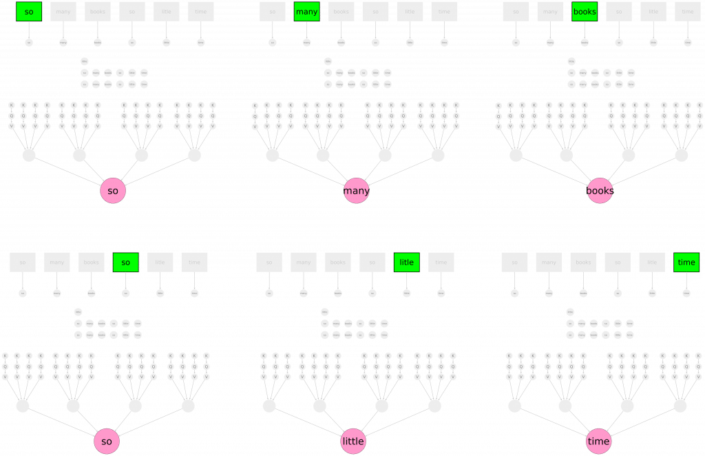
Now we are in a simple world. Our world is a world where we can throw a sentence into a function and expect better, enriched version of that sentence. In fact we can repeat that process many times – we can stack multi-head attention blocks on top of each other – to get further enrichment of input sentence.
Positional encoding
Let’s get back to our reoccurring sentence “So many books so little time”. If we passed this sentence through Multi Head Attention Layer (as introduced so far) – the output for both occurrences of word “so” would be the same – the same embedding vector would be passed for both different occurrences of word “so” and so the same output would be generated. The remedy for this is to add positional information of the word. In Transformer it is achieved by via “positional encoding.”
The simplest possible naive example of positional encoding would be vector of integers – each representing position in the sentence. Authors of Transformer original paper used a bit more complex – yet practical – approach. The formula for positional vector of a word at position $ \text{pos} $ as proposed in Transformer paper is given by:
\[\text{PE}(\text{pos}, 2i) = \sin\left(\frac{\text{pos}}{10000^{2i/512}}\right)\] \[\text{PE}(\text{pos}, 2i+1) = \cos\left(\frac{\text{pos}}{10000^{(2i+1)/512}}\right)\]values of $ i $ goes up to 512 which is also size of embeddings positional vectors are added to.
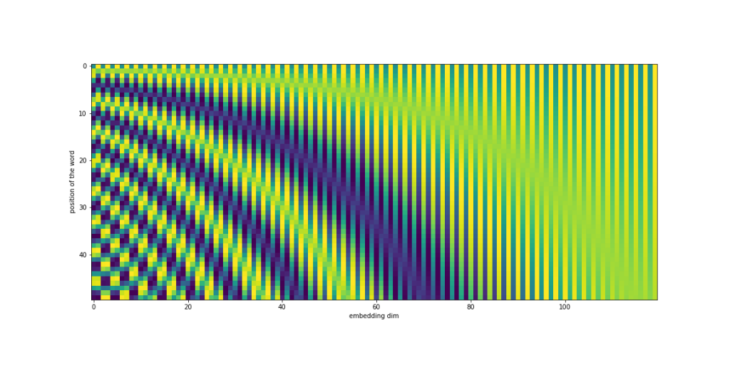
Positional encoding is added to input sentence embedding to ensure positional information being present throughout the Transformer layers.
We chose this function because we hypothesized it would allow the model to easily learn to attend by relative positions, since for any fixed offset k \(\text{PE}_{\text{pos}+k}\) can be represented as a linear function of \(\text{PE}_{\text{pos}}\)
“Attention Is All You Need” paper
(For those curious why they made that choice you can look into Transformer Paper where some justification is provided – there is also a great post on this topic only.)
Transformer Encoder
Originally Transformer was introduced for a problem of language translation with two main components: Encoder and Decoder, both composed of carefully designed Attention Layers stacked on one another. Encoder’s job is to consume a sentence in source language, enhance it and pass it to decoder so it can produce a translation to a target language.
Below you can see original Transformer architecture – with only Encoder being visible. Let’s take a look
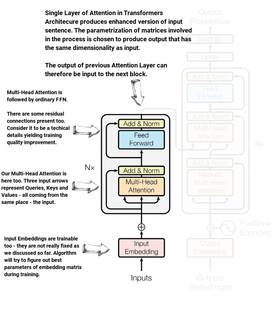
The most important bits here are:
- Transformer Encoder consists of N=6 Attention Layers
- Each Attention Layer produces output of the same size as input – it “enhances” input sentence
- Input Embeddings are trainable (not really fixed word2vec as we tried to imply above – sorry!)
- Residual blocks are present in each Attention Layer
- Transformer Encoder output is feed into each of N decoder Attention Layers
Transformer Decoder
Transformer Encoder is built on top of the concepts we already know – it is positional encoded embedded input sentence crunched through 6 Attention Layers + residual connections and Feed Forward Network.
Transformer Decoder architecture “implements” 3 new ideas – some of which we need to take a closer look at. Let’s take a helicopter view of Decoder architecture and identify these ideas. Then we will focus on each of them separately to fully understand how the whole thing clicks together.
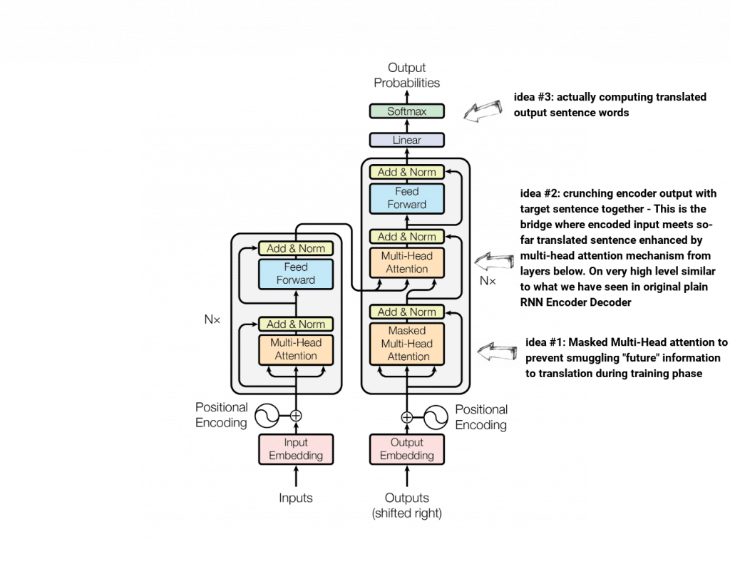
Masked Multi-Head Attention (idea #1)
The final goal of Decoder is – given whole input sentence and sentence translated so far – to compute the next translated word. It is crucial not to smuggle any information about correctly translated from target sentence during training – otherwise our model would be useless – it would learn to copy ground truth to produce translation, facing no ground truth during inference it would fail big time.
The Idea behind masked multi-head attention is to enhance target sentence using previous words only. This is achieved by introducing specially crafted masks that are forcing attention layers to attend to previous words only.
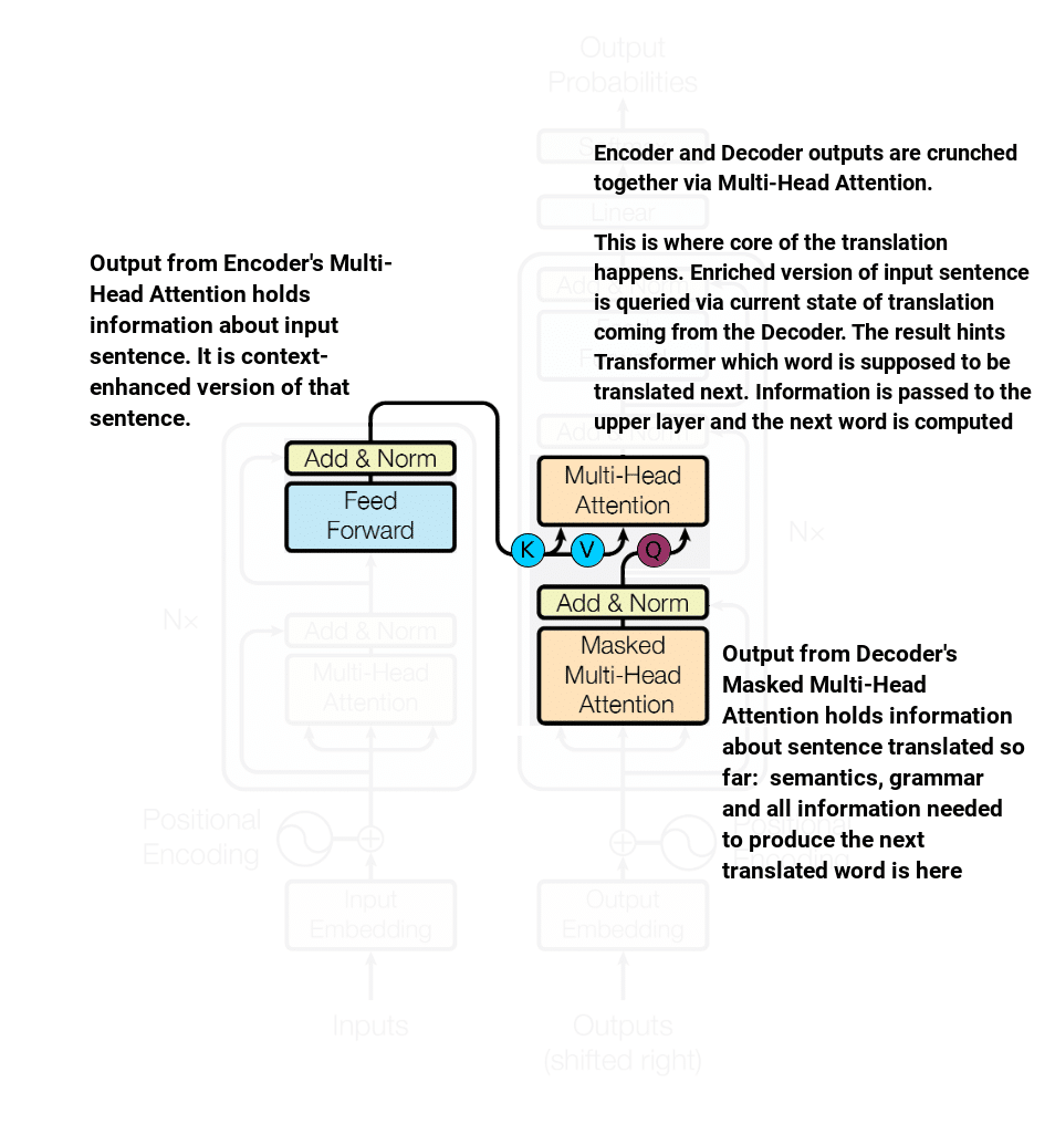
Encoder meets Decoder (idea #2)
Let’s get back to our RNN Encoder-Decoder model for a moment and recall that the very high level idea underlying computing of actual translated word was to combine input sentence context information + information about currently generated translation. Indeed, we used RNN Decoder state (as translated sentence context) and weighted sum of annotations (computed by bi-directional RNN) as information about input sentence. Then these two combined together yielded the next translated word.
Very similar idea applies to Transformer. The only difference is the source of aforementioned information. In Transformer input sentence context (called annotations in RNN – “today” known as keys/values) comes from Encoder while currently translated sentence context (used to be RNN state, now queries) come from Decoder.
Actual translation (idea #3)
This is where actual translation happens. It is rather straightforward – output from decoder/encoder layer is crunched through linear layer to finally go through Softmax that computes probabilities over set of target tokens – meaning actual translation. There are subtle but important details about this part of Transformer like Linear layer sharing weights with trainable embedding layer. More on this can be found in original Transformer paper.
Transformer Model impact on NLP
Transformer Model turned out to have a great impact on NLP.
The Encoder architecture alone was later used in family of BERT language models. First original BERT model was created in 2018. Authors reused Encoder part of Transformer and used it for specially crafted pretext tasks that implied its transfer learning capabilities. Till this day BERT (or tens of its successors) is a major building block of many NLP application in industry.
Another branch of Transformer Model successors reuses its Decoder part. An example of such is generative GPT family of models ‘released’ by OpenAI. The most recent GPT-3 became media favorite after it could mimic human pretty well covering various domains including code generation (code that actually works!).
Summary
That’s all folks. It has been quite a long write-up – I started 8 months ago thinking it would be 3-4 weeks adventure – but life verified it a bit differently. In the meantime, another great, potentially game changer model emerged: MLP Mixer – to my best knowledge its application is mainly Vision – but let’s give it some time to see if this one will kick in as strong as attention-based models.
Anyways, happy to write this summary – I hope maybe this post will help anyone grasping basic intuition about attention mechanism.
Author: int8
Tags: attention mechanism, multi-head attention, neural networks, self-attention, transformer