Solving logistic regression problem in Julia
In this post, we will try to implement gradient descent approach to solve logistic regression problem.
Please note this is mainly for educational purposes and the aim here is to learn. If you want to “just apply” logistic regression in Julia, please check out this one.
Let’s start with basic background.
Logistic regression is a mathematical model serving to predict binary outcomes (here we consider binary case) based on a set of predictors. A binary outcome (meaning outcome with two possible values, like physiological gender, spam/not spam email, or fraud/legitimate transaction) is very often called the target variable, and predictors can also be called features. The latter name is much more intuitive as it is closer to Earth, so to say; it suggests we deal with some sort of objects with known features, and we try to predict a binary feature that is unknown at the time of prediction. The main idea is to predict the target given a set of features based on some training data. Training data is a set of objects for which we know the true target.
So our task is to derive a function that will later serve as a 0/1 labeling machine—a mechanism to produce (hopefully) correct target for a given object described with features. The class of functions we choose to derive the target is called the model. Such a class is parametrized with a set of parameters, and the task of learning is, in fact, to derive these parameters to let our model perform well. Performing well is, on the other hand, measured with yet another function called the goal function. The goal function is what we optimize when we learn parameters for a model. It involves model parameters and training data. It is a function of model parameters and training data with known labels. So the problem of machine learning can be (ignorantly of course) reduced to the problem of estimating a set of parameters of a given class of functions (model) to minimize a given goal function.
Many different models exist with various goal functions to optimize. Today we will focus on one specific model called logistic regression. We will present some basic concepts, formalize data a little bit, and formulate a goal function that will happen to be convex and differentiable (in practice, it means the underlying optimization problem is “easy”).
As we stated before, we will need the following components in our garage.
-
Training data. It is a set of observations/objects you have and you want to learn from. Each observation/object is defined as a set of numbers; each number has a meaning. We model our objects as vectors, so let’s assume the training set is a set of \( N \) vectors \( x \in \mathbb{R}^D \), where \( \mathbb{R} \) is the set of real numbers and \( D \) is the dimensionality of the vectors. It is basically just the number of features an object is described with. We assume each object is described with the same number of features \( D \).
-
Set of labels. For each training example, there is a corresponding binary label. We can model all labels in one structure, a vector again. So let’s assume the target vector to be \( y \in {0,1}^N \).
-
Logistic regression model. This is our model; let’s take a look:
\[f(x, (\beta,\omega)) = \frac{1}{1 + \exp\left(-(\beta + \omega x)\right)}\]where \( x \in \mathbb{R}^D \) is a \( D \)-dimensional vector representing the object under prediction, and \( (\beta, \omega) \) is the set of model parameters. \( \beta \) is a scalar, while \( \omega \) is a \( D \)-dimensional vector of coefficients. Please note that each coefficient corresponds to a single feature, so \( \omega x \) can be seen as a weighted sum of features of \( x \) with \( \beta \) as a free parameter. To get the basic intuition about the reason for such a choice, let’s for now blackbox expression \( \beta + \omega x \) into \( z \) and think of
\[f(z) = \frac{1}{1 + \exp(-z)}\]This function is called the logistic function, and its plot looks like this:
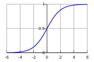
Please note the following properties. The smaller the \( z \), the closer \( f \) to 0, and analogically, the greater the \( z \), the closer \( f \) to 1 (note the minus sign in the formula in case of doubts). Ok, now we can unbox \( z \) again and think of it as a weighted sum again \( \beta + \omega x \). We can also conclude that our model will predict values close to 1 whenever the aforementioned weighted sum is a high positive number, with the opposite holding as well: if the weighted sum is a high negative number, the prediction will be close to 0. That can already provide basic intuition of what we will try to do here. We need to set model parameters in a way that model predictions are close to correct, namely, for 0-labeled data, we want the weighted sum to be as negative as possible, and for 1-labeled data, we wish the opposite. And that brings us to the next puzzle.
-
Goal function: logistic regression optimization problem. The next puzzle is the goal function we wish to optimize. It is going to reflect our intuition of what “learning” means. Once again, what we need is a set of parameters that makes our predictions close to real labels. A common way of representing that is by using likelihood function given by the formula
\[J(\beta, \omega, X, y) = \prod_{i = 1}^{N} f\left(x_{i}, \beta, \omega\right)^{y_{i}} \left(1 - f\left(x_{i}, \beta, \omega\right)\right)^{(1 - y_{i})}\]Even though the formula looks scary, it can be easily explained in an ELI5 fashion. First of all, for any single index \( i \), we in fact deal with either \( f\left(x_{i}, \beta, \omega\right)^{y_{i}} \) or \( \left(1 - f\left(x_{i}, \beta, \omega\right)\right)^{(1 - y_{i})} \). If \( y_i = 0 \) then the first component vanishes; if \( y_i = 1 \), the second one does.
Let’s see what happens to \( f\left(x_{i}, \beta, \omega\right)^{y_{i}} \) depending on the value of \( y_i \):
-
\( y_i = 1 \). If prediction \( f\left(x_{i}, \beta, \omega\right) \) is close to 1, it contributes to \( J \) more.
-
\( y_i = 0 \). If prediction \( f\left(x_{i}, \beta, \omega\right) \) is close to 0, it contributes to \( J \) more.
Then two extremes of function \( J \) are 0 and 1: zero when all predictions are incorrect and 1 in case of correct predictions for all training data points. Our task is then to maximize \( J \) in the parameter space. The convention in the scientific world is to consider any optimization problem as a minimization problem, so in fact, we will try to minimize \( -J(\beta, \omega, X, y) \). Moreover, for mathematical convenience (and practical reasons), we will, in fact, minimize \( - \log\left(J(\beta, \omega, X, y)\right) \). The practical reason can be easily provided: if the number of data points is high enough, the product of many (potentially) small numbers may cause problems with computational precision.
Having all that, we can now wrap our problem in function optimization problem with our function to be optimized given by:
\[\hat{J} = -\log\left(J(\beta, \omega, X, y)\right) = - \sum_{i = 1}^{N} y_{i} \log\left(f\left(x_{i}, \beta, \omega\right)\right) + (1 - y_{i}) \log\left(1 - f\left(x_{i}, \beta, \omega\right)\right)\]Well, believe it or not, but our \( \hat{J} \) function is a convex function of \( \beta \) and \( \omega \). Proof of that is quite long and it uses the fact that a linear combination of convex functions is also convex (so in fact, proof reduces to showing convexity of each component of \( \hat{J} \)).
In the context of optimization, goal function convexity ensures the following: if any local solution is found, it is also a global solution to our problem. This is what makes our problem “easy”.
-
After taking a deep breath, we can now try to solve it. For solving that type of problems, people use gradient descent method. The idea is to start from a random point on a function surface and move towards the gradient at a given point by a certain step \( \alpha \). One can imagine climbing the hill in a locally greedy fashion. Gradient descent method can be described by repeating the following routine:
\[\forall_{i} \quad \omega_{i} = \omega_{i} - \alpha\, \frac{\mathrm{d}\hat{J}}{\mathrm{d}\omega_{i}}\] \[\beta = \beta - \alpha\, \frac{\mathrm{d}\hat{J}}{\mathrm{d}\beta}\]until convergence.
The algorithm will iteratively follow the gradient of the function being optimized and update the current solution with step \( \alpha \). One last piece we miss to implement the algorithm in Julia is the formula for derivatives themselves. This is the matter of calculus:
\[\frac{\mathrm{d}\hat{J}}{\mathrm{d}\omega_{i}} = \dots = \sum_{j=1}^{N} \left( f\left(x_{j}, \beta, \omega\right) - y_{j} \right) x_{ji}\] \[\frac{\mathrm{d}\hat{J}}{\mathrm{d}\beta} = \dots = \sum_{j=1}^{N} \left( f\left(x_{j}, \beta, \omega\right) - y_{j} \right)\]To avoid headaches, I omitted details of that basic (strictly technical) derivation with dots…
Julia Implementation
Let’s now list components we need in our code:
- Main loop. We need a main loop where parameters update takes place.
- Update functions. We need functions to update model parameters in each iteration.
- Goal function. We will need goal function value in each iteration.
- Convergence criterion function (to stop the main loop at some point).
Let’s enclose the main loop within one main function called logistic_regression_learn and add a few helper functions. We will start with simple scaffolding code:
1
2
3
4
5
6
7
8
9
10
11
12
13
14
15
16
17
18
19
20
21
22
23
24
25
26
27
28
29
30
31
32
33
function predict(data, model_params)
    return 1.
end

function goal_function(omega::Array{Float64,2}, beta::Float64, data::Array{Float64,2}, labels::Array{Float64,1})
    return 0
end

function convergence(omega::Array{Float64,2}, beta::Float64, data::Array{Float64,2}, labels::Array{Float64,1}, prevJ::Float64, epsilon::Float64)
    return true
end

function update_params(omega::Array{Float64,2}, beta::Float64, data::Array{Float64,2}, labels::Array{Float64,1}, alpha::Float64)
    omega, beta
end

function logistic_regression_learn(data::Array{Float64,2}, labels::Array{Float64,1}, params::Dict{Symbol,Float64})
    omega = zeros(Float64, size(data,2),1)
    beta = 0.0
    J = Inf
    current_iter = 0
    alpha_step, epsilon, max_iter = params[:alpha], params[:eps], params[:max_iter]

    while !convergence(omega, beta, data, labels, J, epsilon) && current_iter < max_iter
        J = goal_function(omega, beta, data, labels)
        omega, beta = update_params(omega, beta, data, labels, alpha_step)
        current_iter += 1
    end
    model_params = Dict()
    model_params[:omega] = omega
    model_params[:beta] = beta
    return model_params
end
Let’s comment logistic_regression_learn first. Its main goal is to return model parameters that solve the logistic regression problem. Input argument data represents training data points. Labels represent corresponding binary labels. And the last argument params is a dictionary containing all parameters the learning method requires (like gradient descent alpha step, maximal iterations number, and epsilon that is needed to establish convergence).
First few lines within the main function loop (logistic_regression_learn) serve for initialization purposes. We will initialize all of our model (omega and beta) parameters to 0. J will represent the current goal function value. We set it to Infinity to have the worst possible value at the beginning of the algorithm run (it ensures convergence returns false in the first iteration).
Well, we now “only” need to do the boring job of mapping formulas into Julia code. Let’s start with the easiest part, the predict function—with the purpose to predict model output based on given input data and model parameters. It is just logistic function applied on weighted sum of input and model parameters.
1
2
3
function predict(data, model_params)
    1.0 ./ (1.0 + exp(-data * model_params[:omega] - model_params[:beta]))
end
Goal function now:
1
2
3
4
5
function goal_function(omega::Array{Float64,2}, beta::Float64, data::Array{Float64,2}, labels::Array{Float64,1})
    f_partial = 1.0 ./ (1.0 + exp(-data * omega - beta))
    result = -sum(labels .* log.(f_partial) + (1.0 .- labels) .* log.(1.0 .- f_partial))
    return result
end
A few things to observe here. Most importantly, we implicitly chose a certain convention here. We are going to treat data as an array where each row is a single observation. Another detail maybe is that we avoid computing the f function twice and pre-compute it before and store upfront (f_partial).
The code looks quite okay, but it has drawbacks that need attention: goal_function may produce NaN. Let’s try to provoke it:
1
2
3
omega, beta = 750 * ones(1,1), 0.
data, labels = transpose([[1.]]), [1.]
unexpected = goal_function(omega, beta, data, labels)
The value of unexpected in that case is NaN. It’s because
1
exp(-data * omega - beta)
is evaluated to 0, which implies f_partial being evaluated to 1, and finally log(1.0 - f_partial) is then evaluated to -Inf. Corresponding label is zero, and so multiplication of 0 and -Inf results in NaN that is returned. But that is not really expected. Behavior of * operator is problematic here. We need a function that won’t believe in artificial infinity and instead of NaN produce 0. Let’s define that function quickly:
1
2
3
4
5
6
function _mult(a::Array{Float64,1}, b::Array{Float64,1})
    result = zeros(length(a))
    both_non_zero_indicator = ((a .!= 0) .& (b .!= 0))
    result[both_non_zero_indicator] = a[both_non_zero_indicator] .* b[both_non_zero_indicator]
    return result
end
Now we can rewrite the goal function:
1
2
3
4
5
function goal_function(omega::Array{Float64,2}, beta::Float64, data::Array{Float64,2}, labels::Array{Float64,1})
    f_partial = 1.0 ./ (1.0 + exp(-data * omega - beta))
    result = -sum(_mult(labels, log.(f_partial)) + _mult((1.0 .- labels), log.(1.0 .- f_partial)))
    return result
end
Let’s see now:
1
2
3
omega, beta = 750 * ones(1,1), 0.
data, labels = transpose([[1.]]), [1.]
result = goal_function(omega, beta, data, labels)
The result is now correctly evaluated to 0, which is the expected behavior.
Let’s work on the convergence criterion next.
We will use the most intuitive criterion and plan to stop iterating whenever J “practically” stops changing (meaning we are probably very close to the optimal solution). The “practically” part will be expressed by a very small number that will be compared to J change after each iteration. Whenever J does not change by a number greater than epsilon, we stop iterating. The implementation could look like this:
1
2
3
4
function convergence(omega::Array{Float64,2}, beta::Float64, data::Array{Float64,2}, labels::Array{Float64,1}, prevJ::Float64, epsilon::Float64)
    currJ = goal_function(omega, beta, data, labels)
    return abs(prevJ - currJ) < epsilon
end
Additionally, we’ll have a plan B to stop iterating whenever the maximal number of iterations is reached (which could indicate a wrong alpha choice).
The last puzzle is the update function. Let’s first attempt to map formulas into Julia naively:
1
2
3
4
5
6
7
8
9
function update_params(omega::Array{Float64,2}, beta::Float64, data::Array{Float64,2}, labels::Array{Float64,1}, alpha::Float64)
    updated_omega = zeros(Float64, size(omega))
    updated_beta = 0.0
    for i = 1:length(omega)
        updated_omega[i] = omega[i] - alpha * sum((1.0 ./ (1.0 + exp(-data * omega - beta)) - labels) .* data[:, i])
    end
    updated_beta = beta - alpha * sum(1.0 ./ (1.0 + exp(-data * omega - beta)) - labels)
    return updated_omega, updated_beta
end
Naive mapping results in inefficiency. First, note that
1
(1.0 ./ (1.0 + exp(-data * omega - beta)) - labels)
is computed \( D+1 \) times. Let’s compute it once before the loop.
Moreover, the for loop is not needed here. We can instead use basic linear algebra operations to replace it. Note that the summation can be expressed as:
1
2
omega = omega - alpha * (partial_derivative' * data)'
beta = beta - alpha * sum(partial_derivative)
Here’s the updated update_params function:
1
2
3
4
5
6
function update_params(omega::Array{Float64,2}, beta::Float64, data::Array{Float64,2}, labels::Array{Float64,1}, alpha::Float64)
    partial_derivative = (1.0 ./ (1.0 + exp(-data * omega - beta))) - labels
    omega = omega - alpha * (partial_derivative' * data)'
    beta = beta - alpha * sum(partial_derivative)
    return omega, beta
end
Now, let’s put all the pieces together:
1
2
3
4
5
6
7
8
9
10
11
12
13
14
15
16
17
18
19
20
21
22
23
24
25
26
27
28
29
30
31
32
33
34
35
36
37
38
39
40
41
42
43
44
45
46
47
48
function predict(data, model_params)
    1.0 ./ (1.0 + exp(-data * model_params[:omega] - model_params[:beta]))
end

function _mult(a::Array{Float64,1}, b::Array{Float64,1})
    result = zeros(length(a))
    both_non_zero_indicator = ((a .!= 0) .& (b .!= 0))
    result[both_non_zero_indicator] = a[both_non_zero_indicator] .* b[both_non_zero_indicator]
    return result
end

function goal_function(omega::Array{Float64,2}, beta::Float64, data::Array{Float64,2}, labels::Array{Float64,1})
    f_partial = 1.0 ./ (1.0 + exp(-data * omega - beta))
    result = -sum(_mult(labels, log.(f_partial)) + _mult((1.0 .- labels), log.(1.0 .- f_partial)))
    return result
end

function convergence(omega::Array{Float64,2}, beta::Float64, data::Array{Float64,2}, labels::Array{Float64,1}, prevJ::Float64, epsilon::Float64)
    currJ = goal_function(omega, beta, data, labels)
    return abs(prevJ - currJ) < epsilon
end

function update_params(omega::Array{Float64,2}, beta::Float64, data::Array{Float64,2}, labels::Array{Float64,1}, alpha::Float64)
    partial_derivative = (1.0 ./ (1.0 + exp(-data * omega - beta))) - labels
    omega = omega - alpha * (partial_derivative' * data)'
    beta = beta - alpha * sum(partial_derivative)
    return omega, beta
end

function logistic_regression_learn(data::Array{Float64,2}, labels::Array{Float64,1}, params::Dict{Symbol,Float64})
    omega = zeros(Float64, size(data, 2), 1)
    beta = 0.0
    J = Inf
    current_iter = 0
    alpha_step = params[:alpha]
    epsilon = params[:eps]
    max_iter = params[:max_iter]

    while !convergence(omega, beta, data, labels, J, epsilon) && current_iter < max_iter
        J = goal_function(omega, beta, data, labels)
        omega, beta = update_params(omega, beta, data, labels, alpha_step)
        current_iter += 1
    end
    model_params = Dict()
    model_params[:omega] = omega
    model_params[:beta] = beta
    return model_params
end
It’s probably high time to try the code out, but the post is getting too long. I think I’ll stop here and continue evaluation in the future.
But before that, I think we now need some tools for visualization purposes. In the next post, I will try to install and play with Gadfly—a visualization package for Julia.