Chess position evaluation with convolutional neural network in Julia

Posted Apr 2, 2016 Updated Jan 19, 2025

By Kamil

38 min read

In this post we will try to challenge the problem of chess position evaluation using convolutional neural network (CNN) – a neural network type designed to deal with spatial data. We will first explain why we need CNNs then we will present two fundamental CNN layers. Having some knowledge from the inside of the black box, we will apply CNN to the binary classification problem of chess position evaluation using Julia deep learning library – Mocha.jl.

Introduction – data representation

One of the challenges that frequently occurs in machine learning is proper representation of the input data. Ideally, data is desired to be represented in a way that it carries as much information while being digestible for the ML algorithms. Digestibility means fitting in existing mathematical frameworks where known abstract tools can be applied.

A common convenient representation of a single observation is a vector in $\mathbb{R}^n$. Assuming such representation, ML problems may be seen from many different angles – with the benefit of using well-known abstractions/interpretations. One perspective that is very common is the algebraic perspective – having the input data as a matrix (one vector per column), its eigendecomposition or various factorizations may be considered – they both yield important results in the context of machine learning. Set of vectors in $\mathbb{R}^n$ shapes a point cloud – when geometry of such cloud is considered manifold learning methods emerge. A linear model with least squares error has a closed-form solution in the algebraic framework. In all of these cases, representing input data as vectors implies a broad range of tools to handle the problem effectively.

For some domains though it is not obvious how to represent input as vectors while preserving original information contained in the data. An example of such domain is text. A text document is rich in various types of information – there is a semantics and syntax of the text or even personal style of the writer. It is not clear how to represent this unnamed information contained in text. People tend to simplify it and use Bag of Words (BoW) approach to represent text (which completely ignores ordering of words in a document – treats it as a set).

Another domain that suffers from a similar problem is the domain of images. The spatiality of the data is missing when representing images as vectors of dimensionality equal to the total number of pixels. When one represents an image that way the spatial information is lost – the algorithm that later consumes the input vectors is usually not aware the original structure of images is a set of 2-dimensional grids (one matrix for each channel).

So far our neural network has not been aware of two-dimensional nature of input data (MNIST). It could of course find it out itself learning relations between neighboring pixels, but, the fact is, it had no clue so far.

Convolutional neural networks

Convolutional neural networks have been invented to overcome this problem for grid-like structured data (e.g., images). CNNs are designed to take spatial structure (2D + depth) of the data into account and exploit local informativeness of it – meaning that crucial layers of convolutional neural network look for patterns in local regions of the grid (fully connected layers are allowed and very often occur at the output layer). In fact, convolutional neural networks are designed to look for the same pattern in different regions – this combined with proper organization of neurons is a reason for the “convolutional” part of the CNNs name – some groups of neurons when organized in a certain way can be then interpreted as a bunch of convolutions.

Nothing changes on the top level of thinking, for convolutional neural networks, same as for ‘plain’ NNs, each layer serves as a transformation function. It transforms input observation into layer output. One big difference is interpretation of input and output – no matter how they are stored, they are always interpreted as volumes (layers of 2D grids).

To find out more about how CNN transforms input let’s now present new layers of neural networks – these layers are main components of convolutional neural networks.

Convolutional Layer

Just like the layers of regular neural networks, convolutional layer consists of set of neurons. And just like in the case of a regular NN, each neuron consumes its input (high-dimensional) and produces single real output value. The output values of convolutional layer have a nice interpretation when neurons are organized in certain groups. Output of each of these groups can be interpreted as a result of single convolution operation.

Please recall regular neural networks. In such networks each layer consists of a set of neurons and each neuron is fully connected to all of the input vector components – in case of images, any pixel of the image can stimulate any neuron that sees it. That does not hold for convolutional layer. In convolutional layer we also deal with a set of neurons, input, and connections between them but here the connections between neurons and input are constrained. In convolutional layers neurons are organized in groups (please be aware this is just for interpretation purposes) and each neuron in a group is connected to different region of the input such that all neurons in a group contribute to single convolution operation. A single neuron is designed to apply dot product of certain image small region and neuron’s parameters. Moreover, all neurons (contributing to single convolution) share the same set of parameters (this and local connectivity implies significant reduction of number of parameters).

Let’s now point out important information about neurons in a convolutional layer:

each neuron is connected only to a certain region of the input image (image = set of 2D grids)
each neuron—just as in the case of regular neural networks—still performs a dot product
some neurons (those from a group that together perform a convolution) in a given layer share parameters—they all represent one and the same “feature map” applied to different regions of the input grid
The exact organization of connections between neurons and the input is constrained in a way that the convolutional layer’s output can be interpreted as a set of convolutions.

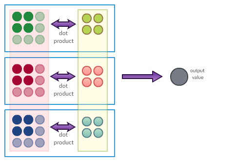
Attempt to visualize single neuron underlying operations of convolutional neural network is presented below:

The left part of the picture represents input. In presented case it consists of 3 (one for each RGB channel) square grids of size 3×3. The middle part of the picture represents neuron parameters (as you can see, our neuron is ‘connected’ to 9 pixel image via 12 parameters, because it only “cares” about one certain local region of the input). Circles being highlighted in input grid are connected to given neuron with the strength given by circles of corresponding color in the middle. This means that our neuron is connected with upper left 2×2 (times 3 channels) region of the input data. It has 12 different parameters. Our neuron sees upper left region of the image – it computes dot product of its parameters and the region values. That’s all.

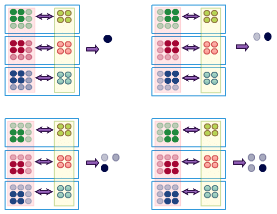
It is important to point out that such a neuron does not exist on its own in convolutional layer. It is an element of certain group of nodes that together perform convolution (more precisely it is a convolution of input data grid and given neurons group’s parameters). What are the other neurons that contribute to convolution operation? Let’s take a look at one example of a group of neurons that contribute to one convolution operation:

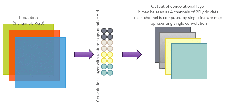
Here, our input consists of three channels, we have one group of 4 neurons that together perform single convolution. It is important to note that single convolution (realized by set of neurons) applied to the input volume (set of 2D grids – like RGB) produces one 2D structure, so it is later a proper input for the next CNN layer.

If you now focus on one single convolution operation (equivalent to set of neurons that performs it) you may interpret it as a feature map sliding over the input. Square window of given size (with depth equal to number of channels) is slid over the input data detecting a pattern (using a dot product as a similarity measure). The instant questions that may emerge now are:

What should be the square size (also called feature map size)?
How to move/slide my feature map over the input?
How to deal with border pixels? How to deal with data from outside the input border?

Asking these questions is justified, and the answers are part of CNNs nature – they are given through hyper-parameters. Each convolutional layer is additionally parametrized with values answering these questions. These parameters though are not something we learn through backpropagation (goal function would not be differentiable if existed in dimensions given by these). We call them hyper-parameters – they are chosen empirically, guessed or they rely on experience, “good practices” or intuition.

Convolutional Layer – parameters and hyper-parameters

Now having a sketch of what convolutional layer is we can take a closer look at the hyper-parameters. Let’s once again point out the most important properties of convolutional layer. It consists of certain number of neurons – each parametrized – all together organized in a specific way so their output can be interpreted as a set of convolutions. Number of neurons and number of parameters per neuron are determined by hyper-parameters.

Let’s list hyper-parameters now and comment how they shape the convolutional layer.

Receptive field size (also known as spatial extent)

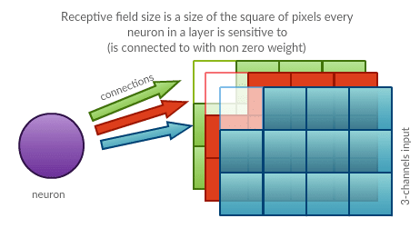
Receptive field size $F$ is the size of the region neurons are sensitive to. Each neuron in convolutional layer is connected to certain region (square) across all channels (input depth). Side of the square (counted in number of pixels) is a parameter. It is shared among all neurons in a layer and it determines the number of parameters for each neuron in a layer. This hyper-parameter also partially determines number of neurons in a layer.

Number of filters/convolutions (also known as depth)

Number of filter maps per layer $N$ is a number being a clue how to organize neurons in convolutional layer such that their output can be interpreted as $N$ convolutions. It determines the output depth and, together with other parameters, number of neurons in a layer. Output depth implies number of “channels” of input transmitted to the next layer. Each convolution produces 2-dimensional output so one can imagine stacking them (creating a deep volume) and passing it to the next layer as input (again, as set of 2D grids).

The stride (step length)

The stride $S$ answers the second question of how to slide a feature map (given by shared parameters of a group of neurons) over the input. Very first thought is to move feature map one pixel at a time (starting from top left part of the input and going in a right/down fashion). One potential problem with that setup is redundancy and it turns out to be good idea to parametrize “stride” or step length. The stride (when parametrized) determines how sparse/dense the neurons are distributed across the input. The greater stride value the greater “gaps” between neurons over the input. Stride (together with other hyperparameters) implies the number of neurons in a convolutional layer.

Picture below presents three (logically) neighbouring neurons (from the same group that performs single convolution) with hyper parameters $S = 2$ (and receptive field $F = 2$) slid over one channel (depth) input of size $4×8$. The stride is accented with violet arrow. The distance between consecutive neurons receptive field (region of images neurons are sensitive to, here highlighted in bluish color) is always 2 (in vertical and horizontal dimension) – this is the stride.

The zero padding amount

Let’s assume input is 2D only (depth = 1) with size $w \times h$ where both $w$ and $h$ are prime numbers. It limits your choice of stride to one single value – 1, dooming you to redundancies (highly overlapping receptive fields of ‘neighbouring’ neurons). One way to overcome this issue is to add zero pixels border around the input. Width of this border is called “zero padding amount” $P$. Zero padding amount determines the output size, too. Sometimes it is crucial to produce output of the same size as input. Zero padding amount is one way of achieving it.

Simplistic visualization of 2 width zero padding added to one channel image matrix (grid) below.

Convolutional layer – hyper parameters choice example

Let’s try to provide an example of convolutional layer now. It is going to be fully determined by the values of hyper-parameters. We can think of convolutional layer being a function of input size and hyper-parameters – these values fully determine the structure of the layer. Receptive field size $F$ tells you how many parameters single neuron needs; input size, stride and zero-padding together imply number of neurons. For given input size, stride and zero-padding there exists only one (if any!) valid number – expressing number of neurons needed in a layer. Be aware that some configurations though may not be valid – like in extreme example above with input size dimensions of length given by prime numbers.

Let’s assume we work on CIFAR-10. The CIFAR-10 dataset consists of 60000 32×32 3-channel images. Let’s try to model the first convolutional layer that operates on that input.

First of all let’s provide a function to determine if given configuration of hyper-parameters is valid. Let’s quickly note that any number of filters is correct if only other hyper-parameters are chosen correctly (valid). We can also only care about width and height of the input image now – as hyper-parameters choice does not depend on input depth. Let’s first point out we will consider more generic case where each of the hyper-parameters may differ for width and height – in other words stride and receptive field can be rectangular and different zero-pixel border may be added vertically and horizontally, in all cases we will index these with small $w$ and $h$ to point out what we refer to (even though in our considerations before we assumed symmetric cases).

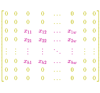
Let’s start from zero padding and note that adding zero pixel values around the image is like changing its original dimensions. After adding zero-padding we have image of size $(W + 2P_w) \times (H + 2P_h)$. Let’s trivially note that now we can only use receptive field of values $F_w \in {1,\dots, (W + 2P_w)}$ and $F_h \in {1,\dots, (H + 2P_h)}$. Receptive field size value reduces number of possible positions of where receptive fields can legally exist – obviously our receptive field can only exist within image size (extended by padding). These positions together (they reference points – like left-corner or center) form a rectangle of size $(W + 2P_w – F_w) \times (H + 2P_h – F_h)$. Now strides $S_w$ and $S_h$ can only be valid if they are a divisor of sizes of that rectangle. We can summarize that and claim that all hyper-parameters meeting the following criteria are valid:

\[\begin{align} ((W + 2P_w – F_w) \mod S_w = 0) \\ ((H + 2P_h – F_h) \mod S_h = 0) \\ (W + 2P_w – F_w > 0) \\ (H + 2P_h – F_h > 0) \end{align}\]

Coming back to our example now, we can conclude that $(N, P_w, P_h, F_w, F_h, S_w, S_h) = (5, 0,0,2,2,2,2)$ is a correct configuration as all requirements above are met, while $(N, P_w, P_h, F_w, F_h, S_w, S_h) = (5,0,0,2,2,4,4)$ is an invalid configuration as $32 + 0 – 2 \mod 4 \neq 0$.

Let’s then choose first configuration and see how many neurons it will produce and so what is the expected output spatial structure. We chose to perform 5 different convolutions on the input image $(N = 5)$ that directly implies output depth to be $5$. As we chose receptive field $F=2$ (symmetrically for width and height) and zero-padding with (symmetric) stride $S=2$ we expect neurons to be spread across the input in non-overlapping fashion (covering the whole image with union of receptive fields though). In this case we expect $5$ layers of $16 \times 16$ neurons resulting in total number of $1280$ neurons. Even though number of neurons is that high, please note that because of parameter sharing among neurons from same group (performing one convolution) number of parameters to optimize for our layer of choice is only $5 \cdot 2 \cdot 2 = 20$.

If we now decided to make our neural network deep – we could add next convolutional layer treating the output as 5-channel input of size 16×16 (possibly activated). In other words convolutional layers are designed to be stacked on top of each other.

Convolutional Layer – summary

Convolutional layer turns out to be set of neurons performing convolutions over input data (across all channels). When creating convolutional layer one has to take care of hyper-parameters that imply number of neurons and number of parameters for given layer. These hyper-parameters determine how to spread neurons across the image, how to ‘slide’ a filter map (implicitly given by certain set of neurons in a layer) over the image – all these result in certain number of parameters that later need optimization (w.r.t. error function – like cross entropy error). Not all configurations of hyper-parameters are correct though, not all make sense – for some configurations we don’t get proper convolutions over the image – and these configurations may be considered invalid. Convolutional layer differs a bit from regular in few aspects: first – some neurons share parameters among each other, neurons are not fully connected to the input (each neuron only cares about local region). Parameters of convolutional layer can be interpreted as filters, when we train convolutional neural network then we in fact try to learn the best set of filters that reveal the goal (like class membership through cross-entropy error). Output of convolutional layer may be interpreted as multi-channel grid (being a ‘proper’ input for the next layer in a network).

Pooling layer – downsampling layer

Another important component of convolutional neural network is pooling layer. Pooling layer is again a transformation layer (as any layer in NN!) that takes volume as input and produces a volume. Pooling layer consists of a set of neurons (this is abstraction of course, different interpretations are there) each neuron is connected to certain image region and performs its underlying transformation. In case of pooling layer each 2D input grid is treated separately. One neuron can only see a region from one 2D grid. Neurons are spread across each channel of 3D input separately. This is different from convolutional layer. In convolutional layer neurons were connected to 3D regions (2D field + depth), here in pooling layer neurons only “care” about input values from single 2D input grid. For each 2D slice of the input there is a separate set of neurons that perform downsampling/pooling.

Neurons in a pooling layer execute an aggregate function $f:F \times F \rightarrow \mathbb{R}$. Function $f$ takes a region (given by receptive field $F$) as input and produces single real value. It can be interpreted as a set of parameterless neurons performing same function $f$. Pooling layer follows the same constraints as convolutional layer when it comes to neurons organization and it uses the same hyper-parameters set except for depth (number of filter maps) – it always produces the volume of the same depth as input.

Types of pooling layer

Depending on exact aggregate $f$ form, pooling layer may have different names. Among many choices, people mainly distinguish the following:

Max pooling layer where $f$ is given by
\[f(X) = \max(x_{i})\]
and $x_i$ are single values of 2D input region $X$ (receptive field).
Average pooling layer where $f$ is given by
\[f(X) = \text{avg}(x_{i})\]
and $x_i$ are single values of 2D input region $X$.
Stochastic pooling layer – where $f$ is given by
\[f(X) = \text{Multinomial}(x_i)\]
and $x_i$ are single values of 2D input region $X$ and multinomial parameters are proportional to values of $X$.

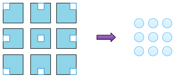
The image above presents the scheme of pooling operation. Each blue square on the left is the same single channel image, white spots represent receptive fields of 9 pooling neurons, for each of receptive fields aggregate function of choice is computed and as a result we get 3×3 2D grid (on the right). If input were multi-channel input, the scheme would involve other channels in a same manner and we would get multi-channel output (volume) as a final result.

Convolutional neural network – summary

What we presented is absolute minimum required to apply convolutional neural network. The whole field is much broader and it is currently one of the most popular research areas. The limited knowledge we now have might still be sufficient to model winning chessboard position – our upcoming task. Single chessboard position is a 2D structure that can be decomposed to separate channels. Let’s then try to apply CNN to the problem of chessboard position evaluation.

Chess position evaluation task

Chess is a two-player board game played on a square 8×8 board (called chessboard). Each of players starts with a set of pieces that are placed on that board. There are 6 types of pieces in chess – each with different characteristics (like set of allowed moves), importance, and strength. The final goal of single chess game is to setup a trap for an opponent’s king – this trap is called “checkmate”. There are two colors of pieces on a chessboard – white and black. White pieces belong to the player who starts the chess game. The other player’s pieces are black. Players move their pieces consecutively until one of the players checkmates the other (or there is a draw or one resigns). In any case, game of chess can be decomposed to a set of pieces configurations on a board – we will further refer to them as positions.

After the game of chess ends (assuming checkmate) – one of the players is the winner. We can therefore take a look at each of the positions that occurred during the game and (optimistically) conclude that every position was a “winning” position for a player who actually won. This is how we are going to compose our dataset. Of course the assumption made here is not entirely correct, especially at the very early stage of the game, it is rather difficult to point anyone’s advantage. Let’s take a shot though*.

*Different approach that turned out interesting is spawk.fish – chess engine that plays in a greedy fashion based on ‘policy network’ – convolutional neural network that predicts ‘the next best move’

Chess position representation

As our final goal is to train convolutional neural network on a set of chessboard positions we need a proper representation of a single position. We want our representation to contain all the information about given position, but we don’t want to use too much of our precious memory. We decided to mix the two following ideas:

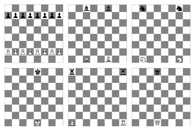
1) First idea is to use separate channel for a single piece type – each single position is represented by 6 channels of 8×8 grid. Each channel only encodes information about pieces of given type. Color of the piece is encoded by a sign. So channels are sparse 8×8 arrays with values from a set ${-1, 0, 1}$. Each position is then represented by 8×8×6 volume being a proper input for convolutional neural network.

Initial chessboard position represented by 6 channels approach (color encodes 1 or -1).

2) Second idea is to extend representation above by adding 1 channel that encodes information about who makes the next move. This is important bit of information when humans evaluate chessboard position.

Our final chessboard representation is then 8×8×7 – 6 channels of 8×8 2D grids with values from ${-1, 0, 1}$ and one additional channel of ones if white is to make the next move or -1s otherwise.

Chess datasets

To conduct the experiments we need to obtain a labeled dataset of chess games positions. Fortunately, with a little help of pgn-extract utility it is possible. To compose final dataset we took the following steps:

Found huge PGN files database.
Chose to download games from years 2014-2015 and beginning of 2016 (Jan – Feb), played by players with rank higher than 2000.
Used pgn-extract utility (available through apt-get) to filter games such that final dataset consists of games finished by checkmate.
Again with pgn-extract we transformed pgn files into epd (Extended Position Description) files – so they contained every position of the games in more friendly format.
Used a bunch of quickly written super ugly and small python scripts to transform EPD files into proper CSV (exact representations are described above).
Transformed CSV files into HDF5 small chunks so it is digestible for Mocha.jl.

Mocha.jl deep learning library

To perform our evaluation task we need a tool that lets us design and train a network. We are going to use Mocha.jl – Julia deep learning library that is inspired by Caffe framework. It supports some of the recent neural networks related techniques and is still under development. The big advantage of using Mocha is the device-independent interface, which means one does not have to be aware where the actual computations take place when designing a network. Mocha.jl goes with a GPUBackend that lets you perform all your heavy computations on GPU.

In Mocha.jl all computations are enclosed within abstractions called “layers”. An instance of Mocha.jl neural network is a sequence of different layers + hyperparameters. To optimize the error function Mocha.jl goes with a solver that determines how to update layers’ parameters after backpropagation step. The final goal is to solve the network using a solver – to cyclically update network parameters optimizing predefined error function.

At the very basic level we can think of three main types of layers:

Input layers – layers that are responsible for consuming the input data, in our case this is going to be HDF5DataLayer that reads HDF5 files and feeds the neural network during training.
Computation layers – layers that are responsible for transforming the data flowing through the network, among many computing layers Mocha.jl includes ConvolutionalLayer, PoolingLayer, and InnerProductLayer. All computing layers require an activation function like ReLU, Sigmoid or Tanh; if no activation function is provided, Identity is used.
Loss layers – defining the function to be optimized – again Mocha.jl includes various types of loss layers – in our case we are mainly interested in BinaryCrossEntropyLossLayer.

Reading the input

First common step for all networks is to prepare the Input Layer. We are going to use a layer called HDF5DataLayer. HDF5DataLayer has quite simple interface – it requires a unique layer name, the source of data and a batch_size.

        
data_layer  = AsyncHDF5DataLayer(name="chess-data", source="train.txt", batch_size=1024, shuffle=true); 
# additionally we want to shuffle our data each time network is fed

train.txt is a file listing all HDF5 chunks intended for a training phase. It is just a text file where each line is a location of the HDF5 file. Because we plan to apply convolutional neural network the underlying HDF5 files by convention have to contain two pieces of data: 4D Tensor called “data” and a 1D vector called “label”. In our case, the tensors dimensions are $8 \times 8 \times 7 \times 500{,}000$ – half a million $8 \times 8 \times 7$ data points while “label” represents binary data labels.

In case of our experiment we decided to divide the dataset into three parts:

17M chessboard positions for training data (2014-2015)
1.5M chessboard positions for validation data (2014-2015)
1.3M chessboard positions for test data (Jan-Feb 2016)*

*Test data was not seen during training and validation, we preprocessed pgn files after model was built to avoid horrible mistake of smuggling test data into training/validation phase

The next thing to do is defining a network architecture. This is the most important part and (at least for us here) it is still a matter of experience, intuition and a gut feeling. As we are not experienced that much, our main result is a consequence of guessing few architectures and comparing the results via common metric.

Network architecture

After few experiments using different layer configurations we noticed the best performing CNN to be the network of the following architecture:

************
*** Mocha.AsyncHDF5DataLayer(train-data)
    Outputs ---------------------------
          data: Blob(8 x 8 x 7 x 1024)
         label: Blob(1 x 1024)
............................................................
*** Mocha.ConvolutionLayer(conv)
    Inputs ----------------------------
          data: Blob(8 x 8 x 7 x 1024)
    Outputs ---------------------------
          conv: Blob(5 x 5 x 400 x 1024)
............................................................
*** Mocha.PoolingLayer(pool1)
    Inputs ----------------------------
          conv: Blob(5 x 5 x 400 x 1024)
    Outputs ---------------------------
         pool1: Blob(3 x 3 x 400 x 1024)
............................................................
*** Mocha.ConvolutionLayer(conv2)
    Inputs ----------------------------
         pool1: Blob(3 x 3 x 400 x 1024)
    Outputs ---------------------------
         conv2: Blob(2 x 2 x 200 x 1024)
............................................................
*** Mocha.InnerProductLayer(ip10)
    Inputs ----------------------------
         conv2: Blob(2 x 2 x 200 x 1024)
    Outputs ---------------------------
          ip10: Blob(70 x 1024)
............................................................
*** Mocha.DropoutLayer(ip10)
    Inputs ----------------------------
          ip10: Blob(70 x 1024)
............................................................
*** Mocha.InnerProductLayer(ip2)
    Inputs ----------------------------
          ip10: Blob(70 x 1024)
    Outputs ---------------------------
           ip2: Blob(1 x 1024)
............................................................
*** Mocha.BinaryCrossEntropyLossLayer(loss)
    Inputs ----------------------------
           ip2: Blob(1 x 1024)
         label: Blob(1 x 1024)
************

The output above is the output from Mocha – ASCII representation of the network architecture. Here is the code generating such a network:

        
      
conv_first_layer  = ConvolutionLayer(name="conv_first_layer", n_filter=400, kernel=(4,4),  bottoms=[:data], tops=[:conv_first_layer]);
pool_layer = PoolingLayer(name="pool", kernel=(2,2), stride=(2,2), bottoms=[:conv_first_layer], tops=[:pool]);
conv_second_layer = ConvolutionLayer(name="conv_second_layer", n_filter=200, kernel=(2,2), bottoms=[:pool], tops=[:conv_second_layer]);
inner_product_layer = InnerProductLayer(name="inner_product_layer", output_dim=70, neuron=Neurons.Sigmoid(), bottoms=[:conv_second_layer], tops=[:inner_product_layer]);
output_layer   = InnerProductLayer(name="output_layer", output_dim=1, bottoms=[:inner_product_layer], tops=[:output_layer], neuron=Neurons.Sigmoid());
loss_layer = BinaryCrossEntropyLossLayer(name="loss", bottoms=[:output_layer, :label]);

drop_layer = DropoutLayer(name="droput_layer", bottoms=[:inner_product_layer], ratio=0.2)

Let’s quickly go through the network layer by layer.

First layer is a ConvolutionLayer with 400 filter maps of size $4 \times 4$ and zero stride (default value). It consumes tensor of size $8 \times 8 \times 7 \times 1024$ and produces a tensor of size $5 \times 5 \times 400 \times 1024$.
The output of first convolutional layer is then consumed by PoolingLayer of $2 \times 2$ receptive field size and $2 \times 2$ stride that produces the output of size $3 \times 3 \times 400 \times 1024$.
Then another ConvolutionLayer follows with 200 filter maps of size $2 \times 2$ and zero stride producing $2 \times 2 \times 200 \times 1024$ tensor.
After that convolution part of the network is over and regular InnerProduct layers kick in. One hidden layer with 70 neurons and sigmoid as activation function and the final output layer that produces the response representing class membership.
The very last layer is the LossLayer that produces error function value and is the base for backpropagation while solving the network later.

DropoutLayer that is present after the first InnerProduct layer is a regularization layer. It is used only during a training phase and its main purpose is to randomly exclude some portion of neuron connections from the training at each iteration. It decreases network expression capacity and may prevent overfitting.

Solving the problem

Now, having our network defined, the underlying problem is an optimization problem. We are after network parameters set that minimize the cross entropy loss. Minimizing the loss alone is not enough, good practice is to divide whole dataset into training set, validation set and test set. Training set is a set that is visible during backpropagation. Validation set is being checked for accuracy every K iterations. The drop of performance on validation set may be a sign of overfitting. To follow that approach let’s create our training network, “validation network” (they both share parameters for most of the layers) and initialize a solver.

        
      
# let's use GPU backend for that task
backend = GPUBackend();
init(backend);

common_layers = [conv_first_layer, pool_layer, conv_second_layer, inner_product_layer, loss_layer];
chessnet = Net("chess-train", backend, [data_layer, common_layers..., drop_layer, loss_layer])
# directory where our experiment output is stored 
exp_dir = "7Dsnapshots-400conv4x4.pool.200conv2x2.ip70.1024batch.dropout0.2";


data_layer_test = AsyncHDF5DataLayer(name="test-data", source="test.txt", batch_size=1024, shuffle=true);
# accuracy layer for binary classification task - default threshold is 0 so we have to define it here to fit our 0-1 labels convention
accuracy_layer = BinaryAccuracyLayer(name="test-accuracy", bottoms=[:output_layer, :label], threshold=0.5);
# test network share "common_layers" 
test_net = Net("chess-test", backend, [data_layer_test, common_layers..., accuracy_layer]);
validate_performance = ValidationPerformance(test_net);


# we are going to use SGD(+momentum) method to update parameters
method = SGD();
# SGD parameters (including momentum, regularization coefficient and learning rate policy 
params = make_solver_parameters(method, max_iter=150000, regu_coef=0.0005, # regularization coefficient 
                                mom_policy=MomPolicy.Fixed(0.9), # momentum is fixed to 0.9 
                                lr_policy=LRPolicy.Inv(0.01, 0.0001, 0.75), # learning rate policy - LR is a function of iter. no 
                                load_from=exp_dir); # possibly load existing snapshots
# instantiate the solver
solver = Solver(method, params);

setup_coffee_lounge(solver, save_into="$exp_dir/statistics.jld", every_n_iter=1000);
add_coffee_break(solver, TrainingSummary(), every_n_iter=300);
add_coffee_break(solver, Snapshot(exp_dir), every_n_iter=2000);
add_coffee_break(solver, validate_performance, every_n_iter=1000);

The last four lines define the diagnostics and other tasks that run during training. Training summary is to be displayed every 300 iterations, snapshot (network parameters’ values) are captured every 2000 iterations and pre-defined validation takes place every 1000 iterations. Finally we can request solving our problem with:

        
      
solve(solver, chessnet)

To measure accuracy we decided to label positions using threshold value $0.5$. After 5 epochs validation accuracy started to decrease slowly for some batches; therefore, we decided to stop the training. In fact already after first epoch we already had test accuracy close to the global top. After five epochs of training we achieved 73.5% validation set accuracy.

Test set accuracy

We set up our solution to store snapshots of the network’s parameters every 2k iterations. We can now load one of the snapshots (the last one actually) to evaluate the network using unseen test data. We were quite fragile about that part and decided to download and preprocess the test data after the model was built.

        
      
using Mocha
# we want to have direct access to data blobs - therefore for prediction we can use CPUBackend
backend = CPUBackend();
init(backend);

# memory layer is a placeholder for our input batches
mem_data = MemoryDataLayer(name="data", tops=[:data], batch_size=1000, data=Array{Float32}(undef, 8, 8, 7, 1000))

# let's build a network that will produce class membership 
run_net = Net("pred", backend, [mem_data, common_layers...])

# feed the network parameters with values learnt during training phase
load_snapshot(run_net, "400-200-70/snapshot-064000");


using HDF5
# read the test data (same structure as input used for training)
h = h5open("D:/chessdataset/2016/test.hdf5")

# here is where we keep predictions 
predictions = Float32[]
# process test data 1000 by 1000 / 130 because there is 1.3M test positions 
for i in 1:130
  # grab current chunk 
  h_chunk = h["data"][:, :, :, (((i-1)*1000 + 1):(1000*i))];
  # feed the network with that chunk 
  get_layer(run_net, "data").data[1][:, :, :, 1:1000] = h_chunk;
  # forward pass 
  forward(run_net);
  # store predictions 
  append!(predictions, run_net.output_blobs[:output_layer].data[:])
end

# get the true labels 
labels = read(h["label"])[:];
test_accuracy = mean(labels .== convert(Array{Float32}, predictions .> 0.5))
# 0.718

Our final test accuracy is 71.8%. That means that we can predict the winner of around 72% of all chess positions for the populations of players playing all types of games (with rank > 2000). It is a bit lower than validation accuracy – we think it might be due to same games (different positions though) being in both training set and validation set.

Chess position evaluation – final results

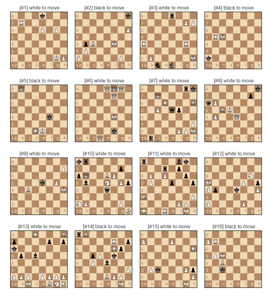
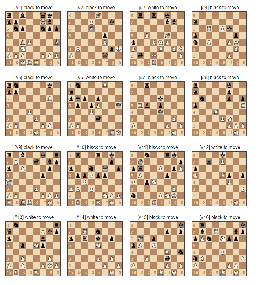
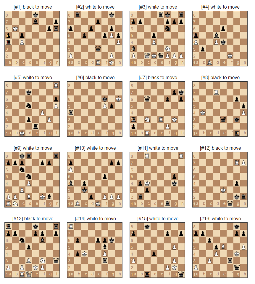
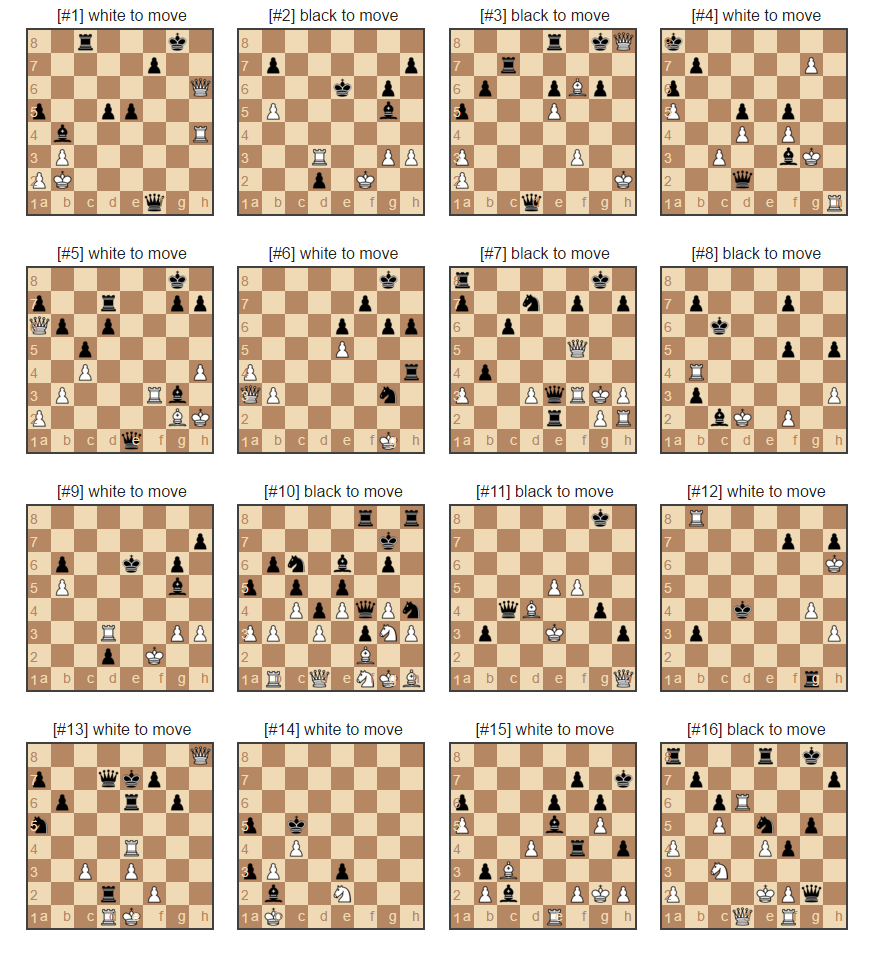
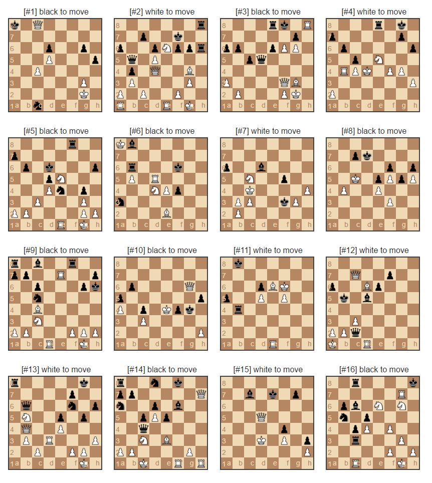
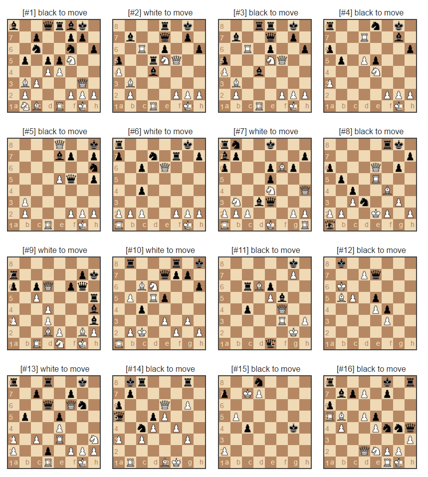
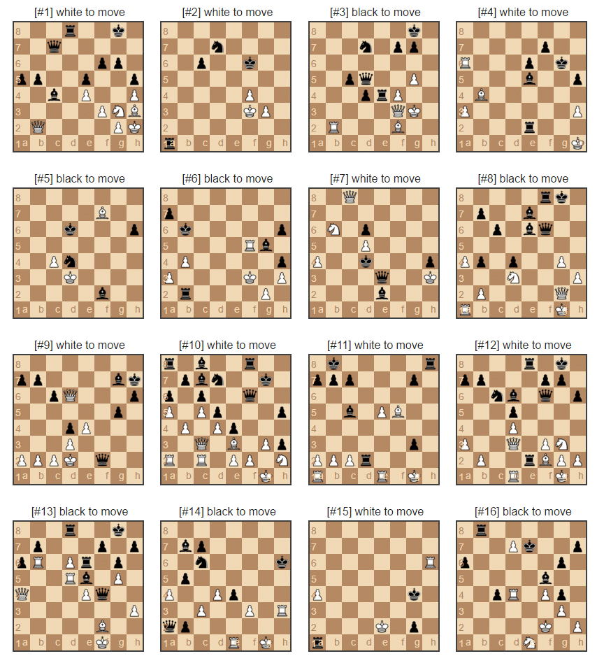
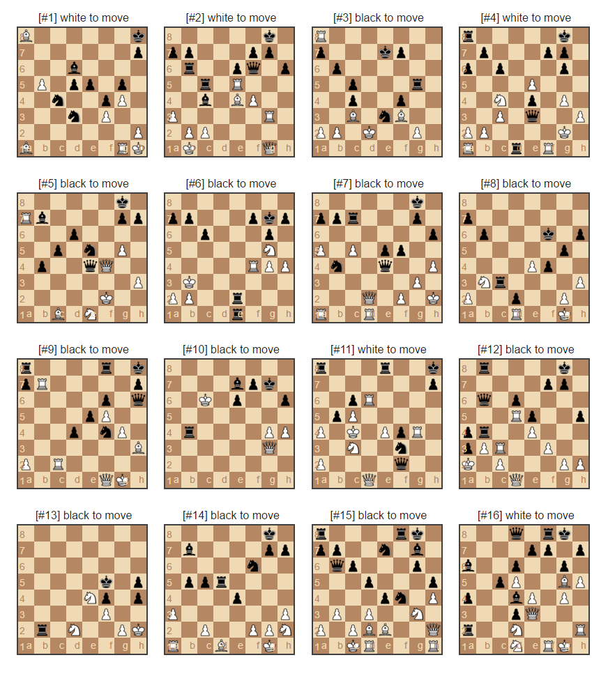
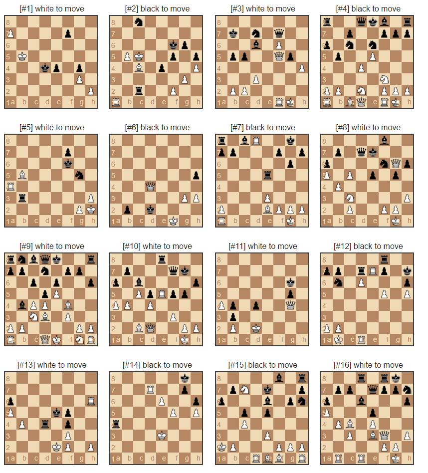
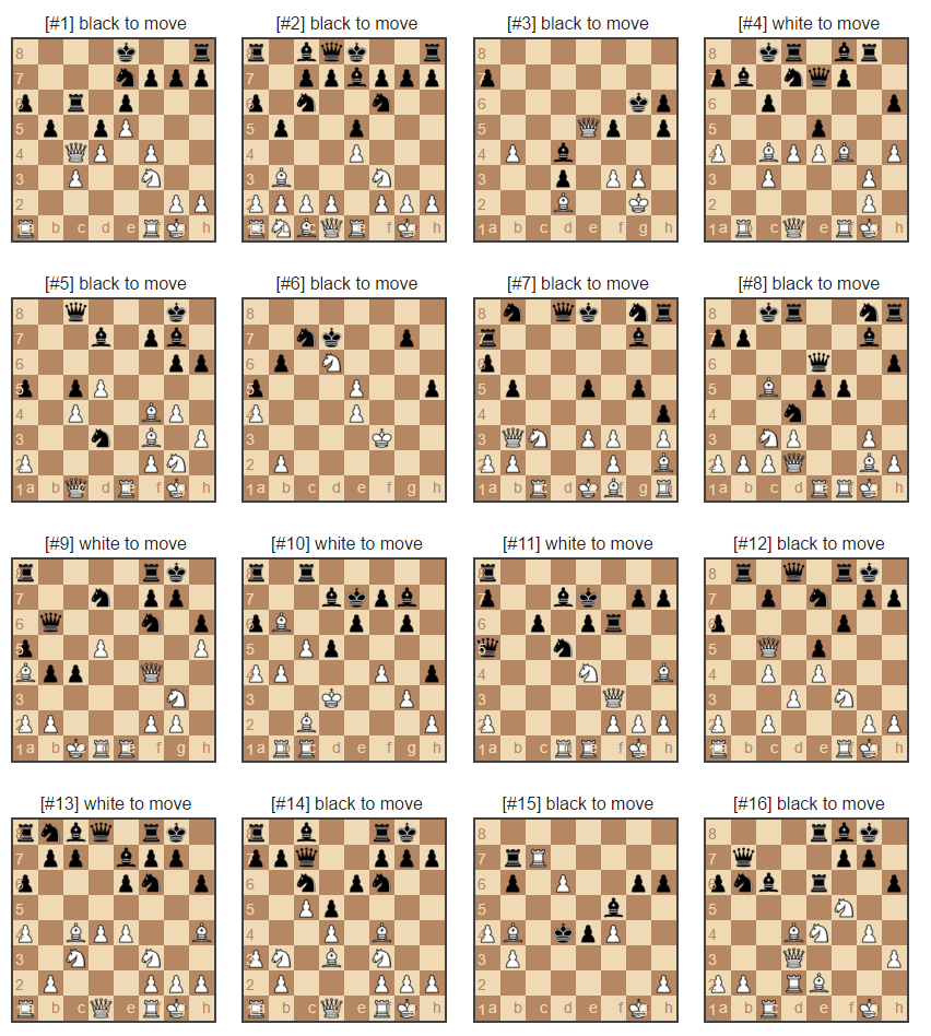
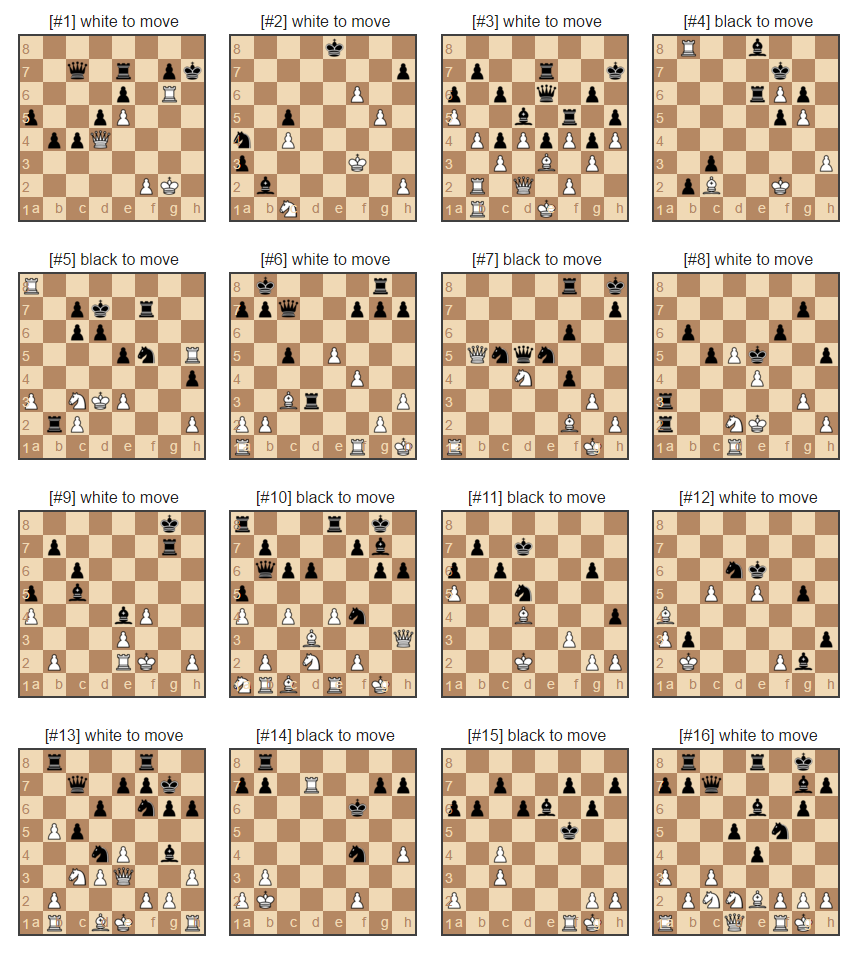
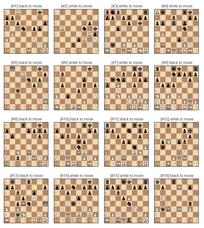
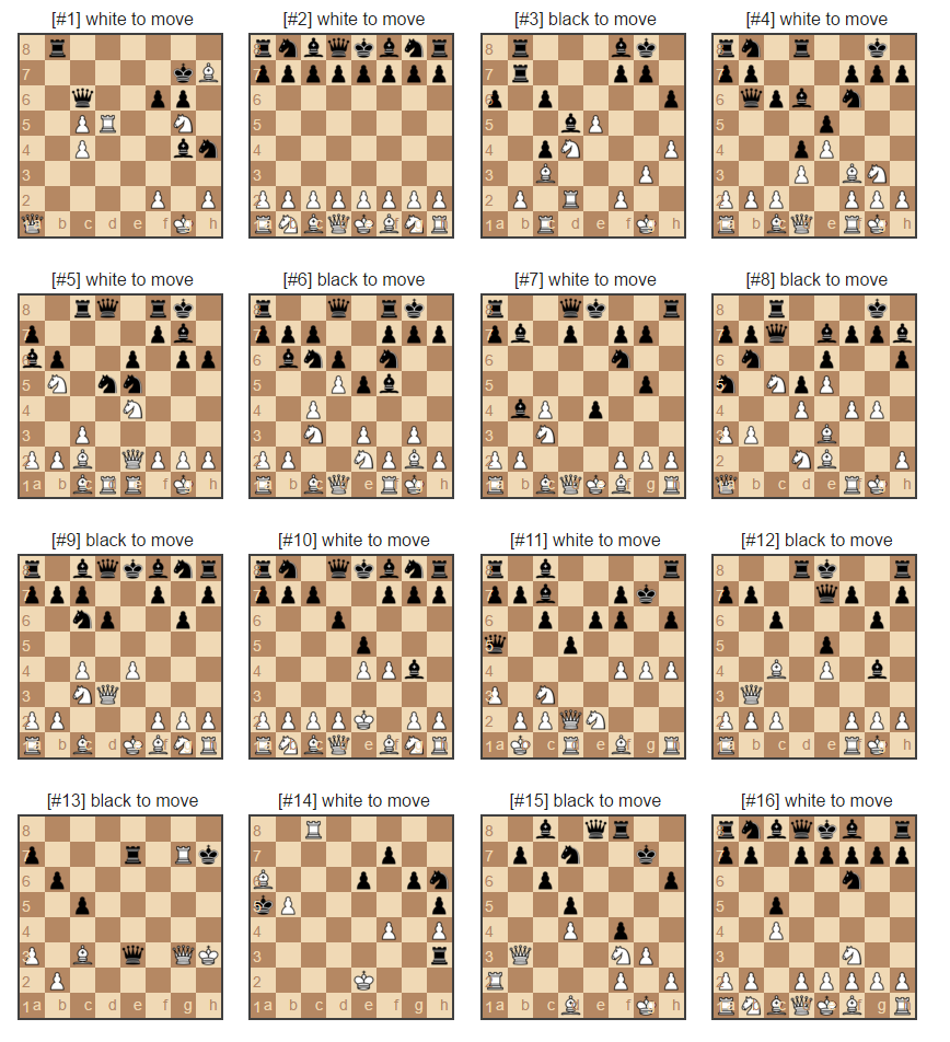
We will now present some of the chessboard positions with true/predicted labels, we will present some of its big mistakes – cases when network is almost sure about the winner while the opponent wins. We will show when it predicts well, and show some examples of chessboard positions the most difficult for our network – when it is unsure about the potential winner.

Our final layer consists of single sigmoid neuron that produces single value between 0 and 1. This value represents chances of white to win. Board position is considered difficult whenever that output value is close to 0.5. When it is polarized towards 0 or 1 it indicates board position being easy to evaluate (at least for our neural network).