Backpropagation from scratch in Julia (part I)
Neural networks have been going through a renaissance recently. After exploding computational power availability (often GPU-based), recent improvements in neural networks initialization (pre-training with RBMs or autoencoders), overcoming vanishing gradient problem in recurrent networks (LSTM), and advances in optimization techniques (AdaGrad, AdaDelta, Adam, and others), neural networks are in the center of attention again. And the attention is tremendous, in fact. Neural networks have won most of the machine learning challenges during the last couple of years. Their bio-inspired nature and human-like roots have caused neural networks’ popularity growth among regular people, too. Friends of mine with no scientific background whatsoever happen to poke me asking if I heard of “singularity” or neural networks by any chance?
Get the code from here
In other words, neural networks can no longer be ignored, and the goal of this post is to catch up a bit and learn basics about them.
Let’s start.
In this series of posts, we will describe step by step how to train a feedforward neural network with the backpropagation algorithm. However, if this is your first attempt to understand backpropagation, I think it is a good idea to take a look at the ELI5/no-math tutorial by Andrej Karpathy. The next step might be to check out this material by Alex Graves (Neural Networks chapter). Another important thing, if you are looking for a near-production-ready implementation, please take a look at Mocha.jl or MxNet.jl if it has to be Julia. Otherwise, one might check out the recently released TensorFlow, Torch7, or Keras.
Here, we will focus on the backpropagation algorithm in the context of a multi-label classification problem. It means we will be given a dataset that is labeled with more than two classes, and our goal will be to classify each dataset entry correctly. Sometimes, to provide an example, we will refer to the MNIST dataset—dataset of images of handwritten digits. Finally, we will run our experiments on MNIST.
One digression: we will use a term “neural network”, but in fact, we will talk about feedforward neural network—a specific type of NN suitable for multi-label classification problem.
What is a neural network?
A neural network is a class of mathematical functions. The functions underneath are parametrized—meaning they behave in a slightly different manner depending on parameter values, but still, they share the same properties and generic behavior. When these parameters are fixed and known, a neural network turns out to be a deterministic composition of functions. In essence, such a network with fixed parameters is a bunch of numbers interpreted in a specific way.
Please take a look at the pseudocode (but don’t commit to it too much—it is just to show a certain duality of the term neural network itself):
1
2
3
4
NeuralNetwork = function(params)
    instance = x -> f(x, params) # Instance of a neural network is the set of function parameters [params] + some constant behaviour [f].
    return instance
end
In this abstract (and practically useless) code, NeuralNetwork is a higher-order function that returns an instance of a neural network given some parameters. Instance of neural network is a function with fixed parameters that takes input from nonfunctional domain and returns output from nonfunctional domain. Such nonfunctional domain-based input could be an image of a digit from the MNIST dataset, and nonfunctional output would be a corresponding label. Most of the time, we will be dealing with a fixed instance of a neural network, but it might be beneficial to realize that a neural network can be interpreted as an abstract entity and therefore can be analyzed in a certain parameter space. This space is what we will try to search at some point in this series of posts. And, in fact, the mysterious backpropagation is just a way of searching such parameter space.
From a more formal perspective, a neural network is a mathematical model. It models certain tiny aspects of reality. How well it models that part of reality depends on its parameters. From that perspective, it does not differ much from a 1D Gaussian distribution (with parameters \( \sigma, \mu \)) that may be used to model a simple distribution of age across a given population.
Before we go deeper, we need to understand what class of mathematical function a neural network expresses. The picture below represents a very first attempt to explain what math hides behind the neural network:
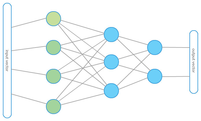
The picture is far from being self-explanatory, so let’s try to explain it a bit going from left to right. This is the right direction as the network final output is computed that way.
On the very left side of the picture, we can see a component called “input vector”. Input vector is a raw data example entering the neural network—it is what the neural network initially sees—its input. In the case of the aforementioned problem of MNIST digits classification, let’s say it is a vector of length 784 (28×28) with each dimension describing a single pixel intensity value.
The next layer of nodes consists of green nodes that represent input vector dimensions. The input vector in our case will be simply put onto the green nodes dimension by dimension to be crunched later by the next layers. In the case of the MNIST dataset, we have 784 green nodes—each for a single pixel intensity value. The next layer of blue nodes represents computing units—these units are called neurons. Neurons process their inputs and produce a single output that is transferred to the neurons in the next layer. Arrows in the picture above represent information flow. They should be read as directed arrows going from left to right. If there is an arrow from node A to node B—it means that whatever comes out from A is an input for B.
Neurons
A neuron is nothing but a function that takes multidimensional input and returns a single real value. That multidimensional input is also an output from the previous network layer—in our toy case from the picture above, each neuron from the second layer will collect inputs from all green input nodes and produce certain output that is later transferred as input to the next layer of neurons.
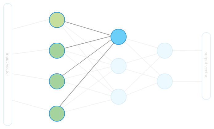
The picture above shows how one neuron gathers input to be processed. When all inputs are ready, the neuron executes its underlying function and produces output that is the input to the next neurons in the next layer. We will refer to the aforementioned function as the “neuron activation function” or simply activation function.
After outputs in the middle layer are all computed, they become input to the next layer consisting of computing nodes again. The result of these computations are finally components of our desired output vector.
One puzzle that is still not solved is a neuron’s underlying activation function. Let’s take a closer look at it. First of all, there is no single correct activation function. We will therefore cover the most popular one called sigmoid activation. Sigmoid activation is parametrized by pair \( \omega, \beta \) and is given by
\[f(x, (\omega, \beta)) = \sigma(w \cdot x + \beta)\]where \( x \) is the function’s input (from the previous layer possibly), \( \omega \) is a vector of parameters of the same size as input, and the dot operation is a dot product (equivalently, we can say that \( \omega \cdot x \) is a linear combination of input, with coefficients given by \( \omega \)). \( \beta \) is a real number called bias (free parameter), and \( \sigma \) is a sigmoid function—a special case of the logistic function known from logistic regression. Let’s try to interpret what happens here in detail and focus on the \( \sigma \) input first:
\[\omega \cdot x + \beta = \omega_{1} x_1 + \omega_2 x_2 + \dots + \omega_n x_n + \beta\]The result of such combination of input vector dimensions is one real (unlimited in range) number. In the case of input coming from raw MNIST example, we would deal with 784 sum components of form
\[\omega_{k} x_{k}\]where \( k \) represents one specific pixel from the 28×28 grid. It means that for each image pixel, the neuron has a corresponding weight to determine how “important” the pixel value is (or how it stimulates the given neuron). The whole combination then expresses the sum of importance of all pixels. This number is then “squashed” to the range \( (0,1) \) by the sigmoid function and serves as input to the next neural network layer. Please note here that if input for a given neuron strongly stimulates it (this happens when the neuron detects a desired pattern), the output value will be high, and so the information of the pattern will be passed further along the network.
Parameters needed for each neuron consist of vector \( \omega \) of the size of the neuron input and a single value \( \beta \) called bias. It is, in fact, input size plus one.
It might be a good idea to think of the recursive nature of the function modeled with our neural network. Each single output value is a composition of activation functions. We will get there soon.
Simple neural network in Julia language
Time to write some code. We will only model blue nodes now—computing nodes—those with sigmoid activation functions. For each node, we will define an input size—so it will “know” what to expect. We will not model “green” input nodes themselves as they will be implicitly present as inputs for the first layer of computing nodes. Our goal then is to implement the sigmoid function applied for a weighted sum of a vector of observations and to store coefficients used to perform that weighted sum—these coefficients are called parameters. Each node will then be a parametrized entity with an underlying “behavior” definition (how to crunch its input).
We could start with something like type definition of a neuron. Such a neuron would have a “parameters” array, input size, and underlying transform function defined. That would work, but we want to take advantage of Julia being a language for scientific computing, so we will be rather going towards representing nodes as whole layers of nodes. It is because computations within a single layer (especially weighted sums!) can be easily enclosed in matrix-vector multiplications, and these operations are highly optimized in Julia. It’s going to be much faster when we think of a layer as our atomic component.
Let’s define sigmoid nodes behavior first:
1
2
3
4
5
6
7
function appendColumnOfOnes(a::Array{Float64,2})
  vcat(a, ones(1, size(a ,2)))
end

function sigmoidNeuronTransformFunction(params, input)
  return 1.0 ./ (1.0 .+ exp(-params * appendColumnOfOnes(input)))
end
First, we define a helper function that adds a row of ones with the purpose to not treat a bias parameter in any special way. sigmoidNeuronTransformFunction is responsible for input transformation inside the sigmoid neuron. This transformation takes two arguments params and input—params is a vector of weighted sum coefficients, and input is an input vector. In fact, its arguments could be matrices too—representing many input vectors entering the whole layer of neurons. That is a very convenient way of treating neural network input/output as it is faster and (for some) more elegant.
Instead of dealing with bias separately, constant value(s) of one(s) is added to the input vector(s), and simple matrix-vector (matrix) multiplication is computed for each layer. Again, this is mainly for speed we get by using basic linear algebra routines.
Quick definition of abstract layer:
1
abstract Layer
We want our types to be abstract as we expect different (than those consisting of sigmoid neurons) types of layers may exist. For now, we will only define a “computing layer”—please note that this is generic with respect to the underlying crunching function.
1
2
3
4
5
6
7
8
9
10
11
type FullyConnectedComputingLayer <: Layer
  inputSize::Int64
  numberOfNeurons::Int64
  parameters::Array{Float64,2}
  transform::Function # we don't define the function directly to get flexibility later

  function FullyConnectedComputingLayer(inputSize, numberOfNeurons, transform::Function)
    parameters = randn(numberOfNeurons, inputSize + 1) # adding one param column for bias
    return new(inputSize, numberOfNeurons, parameters, transform)
  end
end
We defined a type that represents a fully connected computing layer. It consists of a set of nodes (numberOfNeurons) that are connected to all of the nodes from its input layer (inputSize), and it is meant to compute the output and to pass along the result. Parameters are required for later transformation, while transform function is the transformation definition. Please note that parameters is a 2D structure—it is a matrix that holds each single neuron parameters set as one column. This is where we go from neuron to layer perspective.
1
2
3
4
5
6
type NetworkArchitecture
  layers::Array{Layer}
  function NetworkArchitecture(firstLayer::Layer)
    return new([firstLayer])
  end
end
Network architecture defines layer composition. It is important to note that network architecture has only one constructor that always requires the initial layer—a convention we use to initialize the architecture.
1
2
3
4
5
6
function addFullyConnectedSigmoidLayer(architecture::NetworkArchitecture, numberOfNeurons::Int64)
  lastNetworkLayer = architecture.layers[end]
  inputSize = lastNetworkLayer.numberOfNeurons
  sigmoidLayer = FullyConnectedComputingLayer(inputSize, numberOfNeurons, sigmoidNeuronTransformFunction)
  push!(architecture.layers, sigmoidLayer)
end
Given network architecture, we will need to add consecutive layers of neurons. This function adds a fully connected sigmoid layer to the network architecture—this is by far the only neuron type we know.
Let’s now create our first neural network architecture to see what parameters it holds and possibly explain what they mean.
1
2
3
4
sigmoidLayer = FullyConnectedComputingLayer(784, 100, sigmoidNeuronTransformFunction)
architecture = NetworkArchitecture(sigmoidLayer)
size(architecture.layers[end].parameters)
# (100, 785)
After adding a single layer of 100 neurons with sigmoid activation function, we end up with a parameters matrix for that layer of size (100, 785). We deal with 100 vectors of size 785 organized in a matrix. Each vector represents a single neuron—we requested 100 such neurons. Number 785 is the number of parameters for a single neuron. Why 785? As you recall, each neuron is parametrized with a pair \( \omega, \beta \) to be able to compute
\[f(x, (\omega, \beta)) = \sigma(\omega \cdot x + \beta)\]So indeed—in this case, we need 784 weights (one for each pixel) and one free parameter—bias. After adding one more layer to the existing network, we get the following parameter matrix size:
1
2
3
addFullyConnectedSigmoidLayer(architecture, 10)
size(architecture.layers[end].parameters)
# (10, 101)
Again, we requested 10 neurons with sigmoid activation function, but this layer will not “operate on” initial raw input. Input for our new layer is the output from the previous layer. That is why we have (10, 101) size of the parameter matrix. It is because each neuron will only “see” output from previous layer—100 values—as previously we requested 100 neurons. And again, following the same reasoning, we add one extra parameter for each neuron as a bias.
Let’s now make our network compute stuff—we need a function for that:
1
2
3
4
5
6
7
8
function infer(architecture::NetworkArchitecture, input)
  currentResult = input
  for i in 1:length(architecture.layers)
     layer = architecture.layers[i]
     currentResult = layer.transform(layer.parameters, currentResult)
  end
  return currentResult
end
Here, we iterate over layers (note that input is attached at the beginning of the network) and compute each layer output until there is no layer left—meaning we are at the end of the network, and our result is the final network output. Our computing layers are now capable of computing all neuron outputs at once. Let’s try it out.
1
2
3
4
5
6
7
8
9
10
11
12
firstLayer = FullyConnectedComputingLayer(784, 100, sigmoidNeuronTransformFunction)
architecture = NetworkArchitecture(firstLayer)
addFullyConnectedSigmoidLayer(architecture, 50)
addFullyConnectedSigmoidLayer(architecture, 10)
addFullyConnectedSigmoidLayer(architecture, 5)
infer(architecture, randn(784,1)) # we try a single vector now
# 5x1 Array{Float64,2}:
# 0.217054
# 0.681068
# 0.149886
# 0.772127
# 0.458145
As you can see, output vectors consist of 5 components from \( (0,1) \).
Finally, let’s directly write what is the final recursive approximate formula for our neural network function:
\[\begin{align} o_{i}(X) &= o_{i}(o_{i-1}(X)) \\ o_{0}(X) &= X \end{align}\]where \( o_i \) is the output from the \( i \)-th layer of the network and \( X \) is its initial input. As you can see, the neural network is recursive in nature. This will be important when deriving the backpropagation algorithm in the next post.
Conclusions/What next?
Obviously, what we have computed now does not make much sense yet. Our neural network can only produce some random output for now, but please be aware right now there probably exists one specific parametrization that—given a dataset—could produce “correct” labeling. This “one” parametrization is something we are after. Looking for such a “best” parametrization is called “training”. In the next post, we will focus on one specific (and the most popular in case of NN) training technique called backpropagation—backpropagation will turn out to be a certain realization of gradient descent optimization. Before we introduce backpropagation though, we will explain what such a “best parametrization” means. We will use our training dataset and propose an error function that we will try to minimize to achieve the best parametrization.