Random walk vectors for clustering (III)

This is the third post about how to use random walk vectors for clustering. The main idea as was stated before is to represent point cloud as a graph based on similarities between points. Similarities between points are encoded in the form of a matrix, and the matrix is then treated as a weight matrix of a graph. Such a graph is then traversed randomly resulting in a set of random walk vectors (with seed vectors being focused on one different starting point each walk). Each random walk vector represents similarities between points once again—but this time it encodes global dataset shape around given starting point.

In this post we will try to combine many random walk vectors into one matrix that will be used as a data matrix. We will represent each original point as a sequence of numbers that reflect given point’s different cluster memberships. Having that representation we will use NMF clustering technique to cluster these new data points. (I think it might be considered as a type of consensus clustering as well)

We will start with toy datasets to cluster 2D data points of different shapes to finally (next post) work with handwritten digits “MNIST” dataset (previously treated with RBM to reduce its dimensionality). Datasets are available to download: cassini, shapes, smiley, and simplex.

We will need the following routines to make our algorithm work:

• read the datasets
• compute similarity matrix
• compute random walk matrix
• randomly choose seed point
• perform random walk starting from chosen seed
• cluster the data matrix with NMF

Very basic code that does that for us may look like this:

using Distances
using Distributions

function gaussian_similarity(sigma)
  return x -> exp((-x.^2)./(2*sigma^2))
end

function compose_similarity_matrix(dataset::Array{Float64,2}, sigma::Float64)
  gaussian_instance = gaussian_similarity(sigma)
  distance_matrix = pairwise(Euclidean(), dataset)
  gaussian_instance(distance_matrix)
end

function compose_random_walk_matrix(w::Array{Float64,2})
  (w) * diagm(1. ./ (w * ones(size(w,2))))
end

function choose_seed(n::Int64, random_walk_vectors::Array{Float64,2})  
    rand(1:n)
end

function get_random_walk_vectors(random_walk_matrix::Array{Float64,2}, n::Int64, nr_of_random_walks::Int64)
  random_walk_vectors = zeros(size(random_walk_vectors,1), n)
  random_walk_matrix_powered = random_walk_matrix ^ nr_of_random_walks
  k = size(random_walk_matrix, 1)
  seed = choose_seed(k, (1/k) * ones(size(random_walk_matrix,1), 1))
  random_walk_vectors[:, 1] = random_walk_matrix_powered[:, seed]
  for i = 2:n
    seed = choose_seed(k, random_walk_vectors)
    @inbounds random_walk_vectors[:, i] = random_walk_matrix_powered[:, seed]
  end
  return random_walk_vectors
end

function nmf_clustering(data_matrix::Array{Float64,2}, k)
  result = nnmf(data_matrix ./ sum(v, 2), k) 
  nr_of_points = size(data_matrix, 2)
  cluster_membership = zeros(nr_of_points)  
  for i = 1:nr_of_points
     cluster_membership[i] = sortperm(result.W[i, :][:])[end]
  end
  cluster_membership
end

We defined the following components:

• gaussian_similarity function – higher order function returning a gaussian similarity function for given sigma.
• compose_similarity_matrix – returns similarity matrix
• compose_random_walk_matrix – transforms similarity matrix into stochastic matrix
• choose_seed – to randomly select starting vector of random walk; each time we choose a seed point, we take into account random walk vectors produced so far
• get_random_walk_vectors – to generate set of random walk vectors – our temporary goal
• nmf_clustering – to cluster resulting new “data matrix”. This technique is a little bit black-boxed here, of which I am sorry. In essence, the method relies on certain factorization of input matrix (for now please see the details here)—one day I will cover it myself…

Please note that we compute

random_walk_matrix^nr_of_random_walks

which is computationally expensive. One possible improvement would be to sparsify the similarity matrix first. Then we could compute series of matrix-vector multiplications instead of powering the whole matrix. But let’s live with it for now.

Another thing to mention is that each time we choose seed node to start random walk with, we provide all random_walk_vectors computed so far. This gives a chance to use information of where random surfers have been so far, and this again could be a hint for our routine to cleverly choose regions of the graph that were not visited so often.

One possible implementation of this (reflecting very basic intuition) is to choose seed vertex from the probability distribution that is inversely proportional to the sum of the random walk vectors masses in each vertex. Here, we can use Julia package called “Distributions“. Our function could take the following (quite inefficient!) form:

function choose_seed(n::Int64, random_walk_vectors::Array{Float64,2})
    pv = 1 - sum(random_walk_vectors, 2)[:]
    pv = pv / sum(pv)
    c = Categorical(pv)
    rand(c)
end

Toy example – cassini

Let’s try our approach on the toy examples. Let’s start with cassini to see what we gain by using random walk vectors. Let’s read and prepare data points:

cassini = readtable("cassini.csv", separator = ' ', headers = false) 
points = transpose(convert(Array{Float64,2}, cassini[:, 1:2]))
classes = convert(Array{Float64}, cassini[:, 3])
similarity_matrix = compose_similarity_matrix(points, 0.15)
P = compose_random_walk_matrix(similarity_matrix)
v = get_random_walk_vectors(P, 300, 5)

v now holds 300 random walk vectors of length 2000, quick look at some of the resulting vectors:

# using Gadfly 
plot(Geom.point, x = points[1, :], y = points[2, :], color = v[:, 4])
plot(Geom.point, x = points[1, :], y = points[2, :], color = v[:, 5])
plot(Geom.point, x = points[1, :], y = points[2, :], color = v[:, 7])

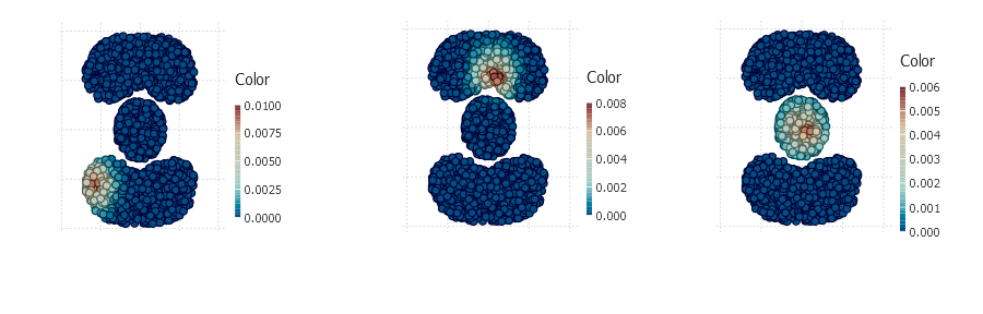
One single vector can be treated as a new dimension that reflects a graph region membership for all points. Matrix v is our new data matrix that contains 2000 points in 300 dimensions.

Let’s now normalize it and use Non-Negative Matrix Factorization based clustering to perform actual clustering. Package NMF will help us here.

# Pkg.add("NMF")
using NMF
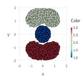
cluster_membership = nmf_clustering(v, 3)
plot(Geom.point, x = points[1, :], y = points[2, :], color = cluster_membership)

Plot produces the final clustering picture:

Application of the same routine onto other toy datasets produces the following results:

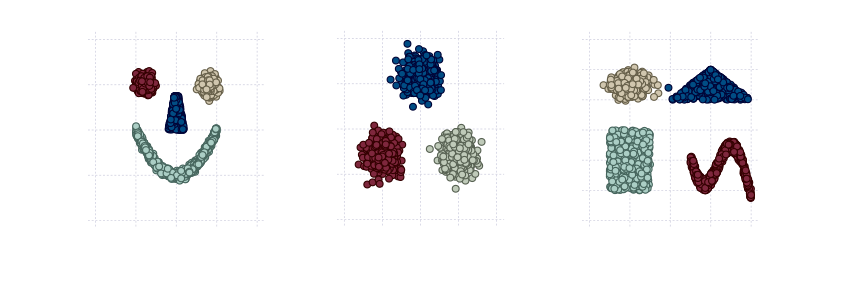
Technique presented in this series of posts passes the exam on toy easily separable datasets. In the next (and final) post we will try the same approach on MNIST dataset and compare it with state-of-the-art k-means algorithm. We will use Clustering package as a source for k-means algorithm and evaluation metric.

---

Author: int8

Tags: clustering, Consensus clustering, NMF, random walks