Automatic differentiation for machine learning in Julia

Posted Jun 16, 2016 Updated Jan 19, 2025

By Kamil

17 min read

Automatic differentiation is a term I first heard of while working on (as it turns out now, a bit cumbersome) implementation of backpropagation algorithm – after all, it caused lots of headaches as I had to handle all derivatives myself with almost pen-and-paper-like approach. Obviously, I made many mistakes until I got my final solution working.

At that time, I was aware some libraries like Theano or TensorFlow handle derivatives in a certain “magical” way for free. I never knew exactly what happens deep in the guts of these libraries though, and I somehow suspected it is rather painful than fun to grasp (apparently, I was wrong!).

I decided to take a shot and directed my first steps towards TensorFlow official documentation to quickly find out what the magic is. The term I was looking for was automatic differentiation.

Introduction – Why do we care at all?

Every problem you solve requires a model that reflects entities involved and interactions between them. Such a model is a simplified mathematical description of reality, a model of your domain. Depending on the exact problem you try to solve, usually, you describe a specific goal in terms of these components/entities. Very often such a goal is given by a function, and the problem is reduced to finding model parameters (numbers that describe your model components’ behavior) that minimize/maximize that function (and so fit your goal best). When you train a supervised neural network, your goal is to minimize error – a difference between predicted outcome and a real one. Similarly, when looking for truncated matrix factorization (like SVD or NMF) your goal is to minimize reconstruction error. In any case, you deal with a goal function that “exists” in a space spanned by your model parameters. That can be attacked from many angles. If you don’t know much about your goal function, you may try to apply simulated annealing, try your luck with genetic algorithms or particle swarm optimization – they all try to heuristically explore a solution space. Very often though, your goal function is designed to be differentiable.

If your goal function is differentiable, one possible way to solve the underlying optimization problem is to apply gradient methods – methods that involve partial derivatives of the function. One popular approach is to apply gradient descent technique that updates your parameters iteratively following the gradient (moving your solution in the direction where your function decreases locally the most).

No matter what exact variant you choose, the essential part of your problem is to compute partial derivatives of your goal function with respect to model parameters. Automatic differentiation is the tool that lets you do it without old-fashioned pen and paper approach (shame on me – I did that couple of weeks ago!).

Input functions – our scope limits

The very first bit that is needed to understand basics of automatic differentiation is the input computer program (function) itself. We will limit our scope here to a certain class of functions that are considered valid (or easy) for AD routines. As we placed ourselves in a context of single goal optimization problem solving (often emerging in machine learning), we will be looking at input functions that require multidimensional input and return one single output*.

f : R^{n} \to R

We want to investigate how to automatically compute gradients of such functions.

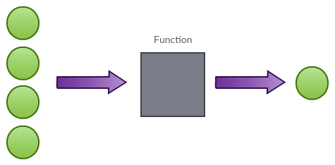
In the picture above, we see a very basic function template of our interest. It accepts multidimensional input and produces one output value. The black box containing our function guts needs to meet certain criteria too. To be proper input for AD routines, it needs to be decomposable to a sequence of differentiable ‘elementary’ functions. By elementary function, we mean unary/binary operators like +, –, *, and functions we know the derivative of (from basic calculus) – like sin, cos, exp, etc*.

It is important to note that automatic differentiation tools are not limited to only these functions, but their focus is much broader. In fact, people differentiate whole computer programs (with “if” conditions, loops, etc.) that are way beyond our limits here.

Forward mode automatic differentiation

Automatic differentiation routines occur in two basic modes. The first one we investigate is called forward mode. Let’s take a look at a simple example function and try to think of how we can compute its partial derivatives (with forward mode AD):

f (x, y) = 2 x + x y^{3} + \sin (x)

As we mentioned before, we want our function to be decomposable to a sequence of differentiable elementary functions. No matter what the exact details are, one can imagine internal representation of function $f$ being given by an abstract expression graph as below:

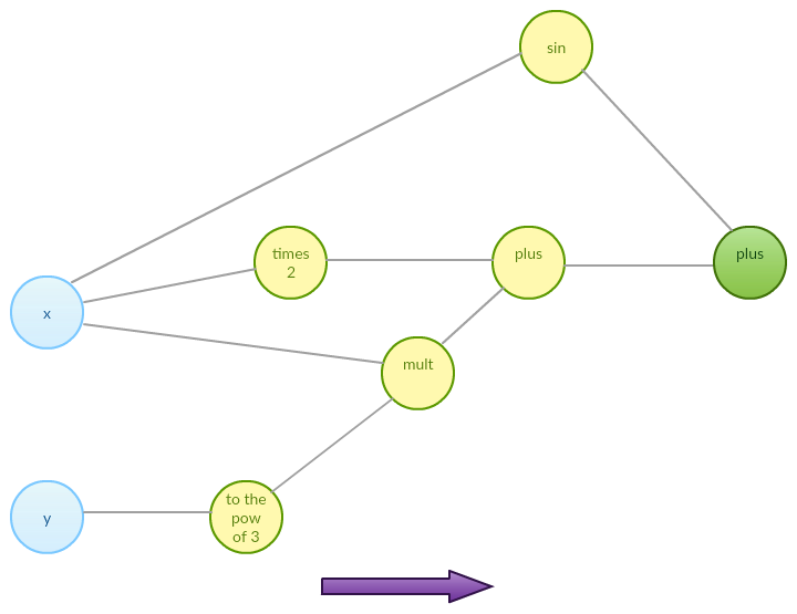
Such expression graph can be further decomposed to a sequence of functions that together compute the final output:

\begin{aligned} f_{1} = x \\ f_{2} = y \\ f_{3} = 2 f_{1} \\ f_{4} = f_{2}^{3} \\ f_{5} = \sin (f_{1}) \\ f_{6} = f_{1} f_{4} \\ f_{7} = f_{3} + f_{6} \\ f_{8} = f_{5} + f_{7} \end{aligned}

Sequence of functions above is derived from the expression graph of our input function $f$ – it decomposes our function into a sequence of functions we know how to handle. Now our function is a sequence of basic operations that change variables’ values. Forward mode automatic differentiation reduces to computing partial derivative with respect to chosen input dimension at given point by differentiating each of the sequence elements forward. Let’s try with point $3, 5$ .

\begin{aligned} f_{1} = 3 & \frac{\partial f_{1}}{\partial x} & = 1 \\ f_{2} = 5 & \frac{\partial f_{2}}{\partial x} & = 0 \\ f_{3} = 6 & \frac{\partial f_{3}}{\partial x} & = 2 \\ f_{4} = f_{2}^{3} = 125 & \frac{\partial f_{4}}{\partial x} & = 0 \\ f_{5} = \sin (3) & \frac{\partial f_{5}}{\partial x} & = \cos (3) \\ f_{6} = 375 & \frac{\partial f_{6}}{\partial x} & = \frac{\partial f_{1}}{\partial x} f_{4} + \frac{\partial f_{4}}{\partial x} f_{1} = 125 \\ f_{7} = 381 & \frac{\partial f_{7}}{\partial x} & = \frac{\partial f_{3}}{\partial x} + \frac{\partial f_{6}}{\partial x} = 127 \\ f_{8} = \sin (3) + 381 & \frac{\partial f_{8}}{\partial x} & = \frac{\partial f_{5}}{\partial x} + \frac{\partial f_{7}}{\partial x} = \cos (3) + 127 \end{aligned}

Please note that differentiation relies on ‘past’ functions’ evaluations – in other words, we need to know the current state of internal variables to compute the next differentiation step (computing $f_{6}$ requires evaluation of $f_{1}$ and $f_{4}$ ). That is why we call this mode of automatic differentiation forward mode. Differentiation happens at the same forward fashion as function evaluation.

One way to go from here is to use Julia metaprogramming capabilities, produce expression graph (possibly based on abstract syntax tree), and construct a program that computes derivatives in a forward mode. That would require a bit of hacking and seems error-prone.

Fortunately, there is another approach that is well adopted now in the world of automatic differentiation. That approach uses function overloading such that our operators and elementary functions accept new data structures called Dual Numbers – these new structures turn out to have certain properties that let you use them to compute function evaluation and its derivative “at the same time” with one pass through expression graph (one forward pass).

Dual Numbers

Dual Numbers are mathematical objects that serve as an extension to real numbers. They have the following form:

a + b ϵ

where $a$ is a real part and $ϵ^{2} = 0$ by definition. Arithmetical operations are defined as follows:

\begin{aligned} (a + b ϵ) + (c + d ϵ) & = (a + c) + (b + d) ϵ \\ (a + b ϵ) (c + d ϵ) & = a c + ϵ (a d + b c) + b d ϵ^{2} = a c + ϵ (a d + b c) \end{aligned}

Moreover, Taylor expansion of $f$ at point $a$ is given by:

f (x) = f (a) + \frac{f^{'} (a)}{1!} (x - a) + \frac{f^{(2)} (a)}{2!} (x - a)^{2} + \dots

Now evaluating the above with $a + b ϵ$ we get:

\begin{aligned} f (a + b ϵ) & = f (a) + \frac{f^{'} (a)}{1!} (b ϵ) + \frac{f^{(2)} (a)}{2!} (b ϵ)^{2} + \dots \\ = f (a) + f^{'} (a) (b ϵ) \end{aligned}

That means we can feed our function $f$ with $a + ϵ$ and expect the resulting dual number to keep function evaluation and its first derivative! All we need to do now is to define Dual Numbers and overload operators we want to compose our function of according to the findings above.

Let’s try to go through our expression graph with dual numbers now and see how to get evaluation and partial derivative with respect to $x$ at point $3, 5$ at once. As we are after partial derivative with respect to $x$ , we are going to feed our function with two dual numbers $x = 3 + ϵ$ and $y = 5 + 0 ϵ$ (with $y$ serving as a constant in that context).

\begin{aligned} f_{1} = 3 + ϵ \\ f_{2} = 5 \\ f_{3} = 6 + 2 ϵ \\ f_{4} = 125 \\ f_{5} = \sin (3 + ϵ) = \sin (3) + ϵ \cos (3) \\ f_{6} = 375 + 125 ϵ \\ f_{7} = 6 + 2 ϵ + 375 + 125 ϵ = 381 + 127 ϵ \\ f_{8} = (381 + \sin (3)) + (\cos (3) + 127) ϵ \end{aligned}

Our function value at $3, 5$ is $381 + \sin (3)$ and its partial derivative with respect to $x$ is $\cos (3) + 127$ and they are both calculated in one run through the expression graph. To compute partial derivative with respect to $y$ the same approach once again may be applied*.

*It reveals a weakness of forward mode automatic differentiation in certain cases. When our function takes many input variables and produces significantly smaller amount of outputs (and this actually happens for most of ML goal functions) we need to evaluate our function $f$ many times with different inputs.*

Dual Numbers in Julia

DualNumbers package is included in current (April 2016) version of Julia. To compute our derivatives all we need to do is:

        
      
using DualNumbers; 

function f(x,y)
  return 2.*x + x.*y.^3 + sin(x)
end

partial_x = f(Dual(3,1), Dual(5,0)) 
# 381.14 + 126.01ɛ
partial_y = f(Dual(3,0), Dual(5,1)) 
# 381.14 + 225.0ɛ

That’s all – our code works already – we don’t need to overload operators and elementary functions as they are already included in DualNumbers package – very basic automatic differentiation technique is already implemented.

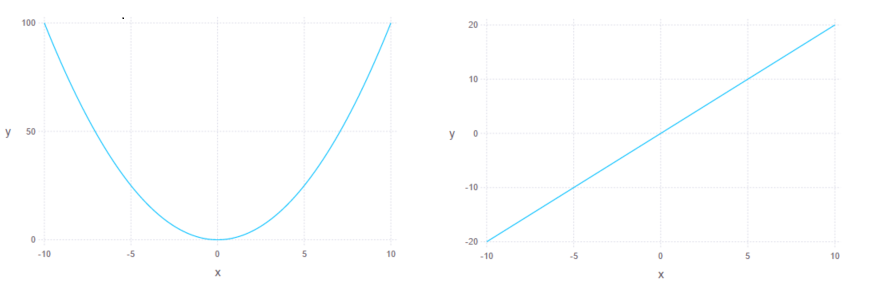
Finally, for a sanity check, let’s try to visualize simple quadratic function and its derivative:

        
      
using DualNumbers; 
using Gadfly 

function f(x)
  return x.^2
end

plot(x =  -10:0.01:10, y = realpart(f([Dual(x,1) for x in -10:0.01:10])), Geom.line)
plot(x =  -10:0.01:10, y = dualpart(f([Dual(x,1) for x in -10:0.01:10])), Geom.line)

Currently Julia community works on a package called ForwardDiff.jl that implements highly optimized forward mode AD methods to compute derivatives, gradients, Jacobians and Hessians of input functions. The whole documentation of ForwardDiff is available here.

Reverse mode automatic differentiation

The main issue with forward mode in our setting is rather practical: whenever we deal with multidimensional goal function – we need to repeat forward pass many times to compute all partial derivatives and that is highly inefficient. Forward mode is much better choice when you deal with function where dimensionality of the domain is much lower than dimensionality of output.

Fortunately, there is a remedy for that – a technique called reverse mode automatic differentiation.

Reverse mode automatic differentiation – basic bits

Formally, reverse mode AD routines rely on the following formula:

\frac{\partial f}{\partial x} = \sum_{\hat{f} \in N_{i n} (f)} \frac{\partial f}{\partial \hat{f}} \frac{\partial \hat{f}}{\partial x}

where $N_{i n} (f)$ means set of nodes connected to node $f$ by incoming (from $f$ perspective) edges in expression tree – in other words these are parents of function node $f$ .

Insert image of expression graph here

Our assumption here is that nodes of our expression tree represent elementary functions – functions easy to handle. Therefore we know analytical form of $f^{'}$ – the only missing puzzle are values of nodes $\hat{f}$ . Therefore to apply differentiation in the reverse mode additional forward pass is needed. It is needed to compute values of each of expression tree nodes. Having that you are able to compute $\frac{\partial f}{\partial \hat{f}}$ .

Applying the same formula recursively for the whole expression tree until input nodes are met is the essential idea of reverse mode automatic differentiation (one could possibly add an extra rule for identity function and treat input nodes as such to get proper recursive formula). What is more important, we only need one forward pass and one backward pass to compute the input function gradient (the crucial components $\frac{\partial f}{\partial \hat{f}}$ are shared across whole gradient).

Implementation-wise, we need expression tree of input function and a function to transform it into a computer program that performs AD routine for us. It is not as easy as it was in case of forward mode AD – although possible with Julia metaprogramming capabilities.

Reverse mode automatic differentiation in Julia

Fortunately we don’t have to risk writing suboptimal code as reverse mode automatic differentiation is already implemented in Julia. The package ReverseDiffSource.jl with rdiff does what we need – it transforms input function into another function that produces derivatives of specified order. It is also well documented – you can find whole documentation here.

Automatic differentiation in action – training autoencoder

Let’s now try to apply automatic differentiation to a real problem – training special kind of neural network called autoencoder. Autoencoders perform dimensionality reduction. One part of the network called encoder tries to encode input data using limited number of dimensions. The remaining part called decoder – is responsible for decoding previously encoded data to preserve the original structure of input as much as possible.

Image below presents a simple template network representing autoencoder:

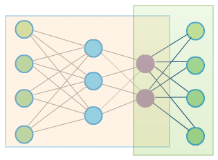
The orangish rectangle is an encoder part of the network. Output of encoding part (purple nodes) is also an input for decoding part (green rectangle). The green nodes are input and output nodes. The goal of the training is to learn identity function – to produce output vectors that are similar (or in ideal world – the same) as input vectors. This goal may be reflected by the following optimization problem (although different formulations exist):

\underset{θ}{\arg \min} \sum_{i}^{n} \sum_{j}^{d} (x_{i j} - F_{θ} (x_{i})_{j})^{2}

where $n$ is number of observations, $d$ is input/output dimensionality and $F_{θ}$ is autoencoder function (network parametrized with $θ$ ). Therefore $x_{i j}$ means $j$ -th component of $i$ -th vector and $F_{θ} (x_{i})_{j}$ is again $j$ -th component of output vector.

To solve that problem we are going to use stochastic gradient descent – the essence of that approach is to compute gradient of our goal function for one single observation and then update the network parameters using simple formula:

θ = θ - α \nabla θ

With automatic differentiation computing a gradient is quite easy task. All we need to do is writing down the goal function. Here let’s make an architectural choice and decide on 3-layers (2-layer encoder + single-layer decoder) network with sigmoid activations, landing with the following error/goal function:

        
      
function autoencoderError(We1, We2 , Wd, b1, b2,  input)
    firstLayer = 1 ./ (1. + exp(-We1 * input - b1))
    encodedInput = 1 ./ (1. + exp(-We2 * firstLayer - b2))
    reconstructedInput = 1 ./ (1. + exp(-Wd * encodedInput))
    return  sum((input - reconstructedInput).^2)
end

Let’s also define two helper functions to initialize network parameters and load input data – in our simple experiment it is a MNIST dataset:

        
      
function readInputData()
    a,_ = MNIST.traindata();
    A = a ./ 255;
    return A;
end

function initializeNetworkParams(inputSize, layer1Size, layer2Size, initThetaDist)
    We1 =  rand(initThetaDist, layer1Size, inputSize); b1 = zeros(layer1Size, 1);
    We2 =  rand(initThetaDist, layer2Size, layer1Size); b2 = zeros(layer2Size, 1);
    Wd = rand(initThetaDist, inputSize, layer2Size);
    return (We1, We2, b1, b2, Wd);
end

Having these two we can finally proceed to the most important part – training:

        
      
using MNIST; # if not installed try Pkg.add("MNIST")
using Distributions; # if not installed try Pkg.add("Distributions")
using ReverseDiffSource; # if not installed try Pkg.add("ReverseDiffSource")

A = readInputData(); # read input MNIST data 
input = A[:,1]; # single input example is needed for AD routine
We1, We2, b1, b2, Wd = initializeNetworkParams(784, 300, 100, Normal(0, .1)); # 784 -> 300 -> 100 -> 784 with weights normally distributed (with small variance)
autoencoderGradients = rdiff(autoencoderError, (We1, We2, Wd, b1, b2, input), ignore=[:input]); 
# autoencoderGradients now holds a function that computes a gradient (ignoring input means it won't calculate derivatives with respect to input)


function trainAutoencoder(epochs, inputData, We1, We2, b1, b2, Wd, alpha)
    for _ in 1:epochs
        for i in 1:size(inputData,2)
            input = A[:,i]
            partialDerivatives = autoencoderGradients(We1, We2, Wd, b1, b2, input);
            partialWe1, partialWe2, partialWd, partialB1, partialB2 = partialDerivatives[2:6];
            We1 = We1 - alpha * partialWe1; b1 = b1 - alpha * partialB1;
            We2 = We2 - alpha * partialWe2; b2 = b2 - alpha * partialB2;
            Wd = Wd - alpha * partialWd;
        end
    end
    return (We1, We2, b1, b2, Wd)
end

We1, We2, b1, b2, Wd = trainAutoencoder(4, A,  We1, We2, b1, b2, Wd, 0.02);

The last line will run through 4 epochs and return final parameter values. The main point here is that we don’t have to compute gradients ourselves. All we need to focus on is expressing the problem we are about to solve and – if only it is differentiable – rdiff does the job for us.

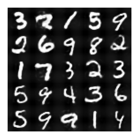
Training autoencoder – results

After four epochs we get the following results for random training set inputs: [Left: input; Right: output]

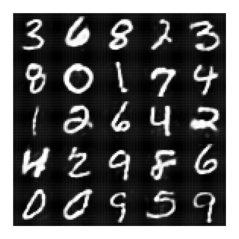
And reconstructions as below for random test set inputs: [Left: input; Right: output]

In addition to nice reconstructions, the other advantage of autoencoders is their ability to capture dataset features given by ‘encoding part’ of the network. These features can be further used for neural networks pre-training or direct data representation for other tasks like classification.

Summary

In this post we went through Forward mode AD and so Dual numbers and reverse mode AD with example of Julia implementation usage for autoencoder network. Training such a network reduced to defining a goal without designing gradient computing routine. AD library did this part for us.

Automatic differentiation seems like a very practical tool although still in a starting phase in Julia – still I keep my fingers crossed for the whole autodiff project in Julia and hope to see more progress in the future.

Automatic differentiation

This post is licensed under CC BY 4.0 by the author.