Neural Networks in Julia – Hyperbolic tangent and ReLU neurons
Our goal for this post is to introduce and implement new types of neural network nodes using Julia language. These nodes are called ‘new’ because this post loosely refers to the existing code.
So far we introduced sigmoid and linear layers and today we will describe another two types of neurons. First we will look at hyperbolic tangent that will turn out to be similar (in shape at least) to sigmoid. Then we will focus on ReLU (rectifier linear unit) that on the other hand is slightly different as it in fact represents non-differentiable function. Both yield strong practical implications (with ReLU being considered more important recently – especially when considered in the context of networks with many hidden layers).
What is the most important though, adding different types of neurons to neural network changes the function it represents and so its expressiveness, let’s then emphasize this as the main reason they are being added.
Hyperbolic tangent layer
From the biological perspective, the purpose of sigmoid activation function as single node ‘crunching function’ is to model passing an electrical signal from one neuron to another in brain. Strength of that signal is expressed by a number from $(0,1)$ and it relies on signal from the input neurons connected to the one under consideration. Hyperbolic tangent is yet another way of modelling it.
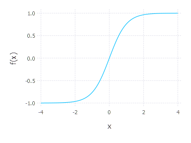
Let’s first take a look at the form of hyperbolic tangent:
\[f(x) = \frac{\mathrm{e}^x – \mathrm{e}^{-x}}{\mathrm{e}^x + \mathrm{e}^{-x}}\]Shape of hyperbolic tangent is similar to sigmoid:
but its values come from different range that includes negative values $(-1,1)$. Derivative of hyperbolic tangent is given by:
\[\frac{\partial f}{\partial x} = 1 - f(x)^2\]Knowing underlying crunching function of our new neuron and its derivative we can now add it to our current implementation in Julia. First we will re-organize our code a bit. We will generalize existing Julia functions addFullyConnectedSigmoidLayer and addFullyConnectedLinearLayer and change it to one function addFullyConnectedLayer – it will require the logic (crunching and derivative functions) as input. Another thing to change is a function buildNetworkArchitecture* function that assumes architecture to consist of sigmoid or linear neurons only. We need to add flexibility of choosing different types of computing nodes. Let’s take a look at the changes we want to make:
1
2
3
4
5
6
7
8
9
10
11
12
13
14
15
16
17
18
19
20
...
function addFullyConnectedLayer(architecture::NetworkArchitecture, numberOfNeurons::Int64, functionsPair::(Function,Function))
 lastNetworkLayer = architecture.layers[end]
 inputSize = lastNetworkLayer.numberOfNeurons
 layer = FullyConnectedComputingLayer(inputSize, numberOfNeurons, functionsPair[1], functionsPair[2])
 push!(architecture.layers, layer)
end
...

function buildNetworkArchitecture(inputSize, layersSizes, layersFunctions::Array{Function})

  firstLayer = FullyConnectedComputingLayer(inputSize, layersSizes[1], layersFunctions[1]()[1], layersFunctions[1]()[2]);
  architecture = NetworkArchitecture(firstLayer);
  for i in 2:(length(layersSizes))
    addFullyConnectedLayer(architecture, layersSizes[i], layersFunctions[i]());
  end
  addSoftMaxLayer(architecture)
  return(architecture)
end
...
First we change functions that add computing layer to neural network, we now expect pair of functions instead of two functions as it was before. Now, when building the network architecture we specify input size and sizes of consecutive neuron layers, additionally we specify underlying layer functions pairs (transform for forward and derivative for backward pass). Please also note that function pairs are given by higher order functions that return these function pairs. It is rather cumbersome at first but it works and may seem more elegant later (I’m aware that introducing a type would be a solution here – but let’s have it as it is now).
Having these functions defined like that we can now rewrite sigmoid and linear layers. It reduces to defining function pairs and higher order function called “layer”:
1
2
3
4
5
6
7
8
9
10
11
12
13
14
15
16
17
18
19
20
21
22
23
24
25
...
function sigmoidNeuronTransformFunction(params, input)
  return 1.0 ./ (1.0 .+ exp(-params * appendColumnOfOnes(input)))
end

function sigmoidNeuronDerivativeFunction(input)
  return  input .* (1 - input)
end

function sigmoidComputingLayer()
  return (sigmoidNeuronTransformFunction, sigmoidNeuronDerivativeFunction)
end

function identityNeuronTransformFunction(params, input)
   return params * appendColumnOfOnes(input)
end

function identityNeuronDerivativeFunction(input)
  return  1
end

function linearComputingLayer()
  return (identityNeuronTransformFunction, identityNeuronDerivativeFunction)
end
...
Now if we want to build architecture that consists of sigmoid layers, this is the way to do it:
1
2
trainingData, trainingLabels, testData, testLabels = loadMnistData()
architecture = buildNetworkArchitecture(784, [50,20,10], [sigmoidComputingLayer, sigmoidComputingLayer, linearComputingLayer])
Finally adding tanh layer reduces now to adding three functions as follows:
1
2
3
4
5
6
7
8
9
10
11
12
13
14
...
function tanhNeuronTransformFunction(params, input)
   x = params * appendColumnOfOnes(input)
   return tanh(x) # we use built-in Julia version of tanh
end

function tanhNeuronDerivativeFunction(input)
  return  1 .- input.^2
end

function tanhComputingLayer()
  return (tanhNeuronTransformFunction, tanhNeuronDerivativeFunction)
end
...
Now we can use tanh and linear computing layer when constructing our network. For example:
1
2
trainingData, trainingLabels, testData, testLabels = loadMnistData()
architecture = buildNetworkArchitecture(784, [50,200,10], [tanhComputingLayer, tanhComputingLayer, linearComputingLayer])
Rectifier linear units – ReLU layer
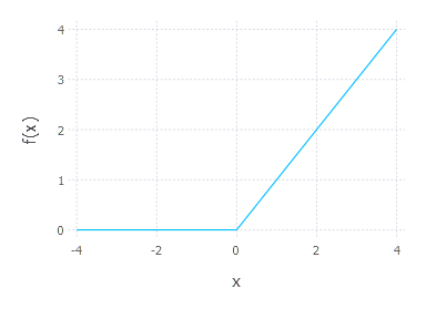
Rectifier linear units are yet another types of nodes in neural networks. Their popularity has grown recently after successful application of ReLU in deep neural networks. The main reason why ReLU is suitable for deep networks is its resistance to “vanishing gradient problem” – practical problem that occurs when backpropagation algorithm is applied for deep neural networks. ReLU neurons’ activation is given by:
\[f(x) = \mathrm{max}(0, x)\]where $x$ can again be seen as a linear combination of input and ReLU neuron parameters.
Function under consideration yields one problem – it is not differentiable at $0$, therefore there is no analytical derivative of that function in zero – still, people use ReLU with success assuming derivative at $0$ to be zero. We can assume same thing and write
\[\frac{\partial f}{\partial x} = \begin{cases} 1 & \quad \text{if } x > 0\\ 0 & \quad \text{otherwise} \end{cases}\]Again, adding that simple implementation to our current code is straightforward. Again we “just” add three functions like:
1
2
3
4
5
6
7
8
9
10
11
12
13
14
...
function reluNeuronTransformFunction(params, input)
   x = params * appendColumnOfOnes(input)
   return x .* (x .> 0)
end

function reluNeuronDerivativeFunction(input)
   return convert(Array{Float64,2}, input .> 0)
end

function reluComputingLayer()
  return (reluNeuronTransformFunction, reluNeuronDerivativeFunction)
end
...
and now we have flexibility of using four different computing layers in our neural networks.
Quick experiments
ReLU neurons
Let’s quickly try out if we really can use our new types of neurons.
1
2
3
4
5
6
7
8
9
10
11
12
13
14
15
16
trainingData, trainingLabels, testData, testLabels = loadMnistData()
architecture = buildNetworkArchitecture(784, [50,10], [reluComputingLayer, linearComputingLayer])
crossEntropies = Float64[]
batchSize = 20
for i = 1:10000
   minibatch = collect((batchSize*i):(batchSize*i +batchSize)) % size(trainingLabels,2) + 1 # take next 20 elements
   learningUnit = BackPropagationBatchLearningUnit(architecture, trainingData[:,minibatch ], trainingLabels[:,minibatch]);
   updateParameters!(learningUnit, 0.1)
   if i % 100 == 0  # this one costs so let's store entropies every 100 iterations
     push!(crossEntropies, crossEntropyError(architecture, trainingData, trainingLabels))
   end
end
plot(x = 1:length(crossEntropies), y = crossEntropies, Geom.line, Guide.xlabel("iterations (/100)"), Guide.ylabel("error"))
inferedOutputs = infer(architecture, testData)
mean(mapslices(x -> indmax(x), inferedOutputs ,1)[:]  .==  mapslices(x -> indmax(x), full(testLabels),1)[:])
# 0.955
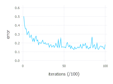
As we can see, when using ReLU neurons accuracy is comparable to the same architecture with sigmoids in hidden layer. It is much less stable though.
Tanh neurons
1
2
3
4
5
6
7
8
9
10
11
12
13
14
15
16
trainingData, trainingLabels, testData, testLabels = loadMnistData()
architecture = buildNetworkArchitecture(784, [50,10], [tanhComputingLayer, linearComputingLayer])
crossEntropies = Float64[]
batchSize = 20
for i = 1:10000
   minibatch = collect((batchSize*i):(batchSize*i +batchSize)) % size(trainingLabels,2) + 1 # take next 20 elements
   learningUnit = BackPropagationBatchLearningUnit(architecture, trainingData[:,minibatch ], trainingLabels[:,minibatch]);
   updateParameters!(learningUnit, 0.1)
   if i % 100 == 0  # this one costs so let's store entropies every 100 iterations
     push!(crossEntropies, crossEntropyError(architecture, trainingData, trainingLabels))
   end
end
plot(x = 1:length(crossEntropies), y = crossEntropies, Geom.line, Guide.xlabel("iterations (/100)"), Guide.ylabel("error"))
inferedOutputs = infer(architecture, testData)
mean(mapslices(x -> indmax(x), inferedOutputs ,1)[:]  .==  mapslices(x -> indmax(x), full(testLabels),1)[:])
# 0.9548
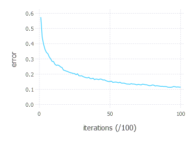
Using tanh yields similar results to ReLU and sigmoid, tanh and sigmoid seem to be more stable than ReLU.
What’s next?
We do not present any more experiments in this post as it makes more sense to introduce different optimization techniques first (coming soon in the next post) and provide experiments results cumulatively, later.


