Optimization techniques comparison in Julia: SGD, Momentum, Adagrad, Adadelta, Adam

In today’s post we will compare five popular optimization techniques: SGD, SGD+momentum, Adagrad, Adadelta, and Adam – methods for finding local optimum (global when dealing with convex problems) of certain differentiable functions. In the experiments conducted later in this post, these functions will all be error functions of feed-forward neural networks of various architectures for the problem of multi-label classification of MNIST (dataset of handwritten digits). In our considerations, we will refer to what we know from previous posts. We will also extend the existing code.

Stochastic gradient descent and momentum optimization techniques

Let’s recall the stochastic gradient descent optimization technique that was presented in one of the last posts. Last time we pointed out its speed as a main advantage over batch gradient descent (when the full training set is used). There is one more advantage, though. Stochastic gradient descent tends to escape from local minima because the error function changes from mini-batch to mini-batch, pushing the solution to be continuously updated (a local minimum for the error function given by one mini-batch may not be present for another mini-batch, implying a non-zero gradient).

Traversing through error differentiable functions’ surfaces efficiently is a big research area today. Some of the recently popular techniques (especially in application to neural networks) take the gradient history into account such that each “move” on the error function surface relies a bit on previous ones. An example of childish intuition of that phenomenon might involve a snowball rolling down a mountain. Snow keeps attaching to it, increasing its mass and making it resistant to getting stuck in small holes on the way down (because of both the speed and mass). Such a snowball does not teleport from one point to another but rather rolls down within a certain process. This infantile snowy intuition may be applied to the gradient descent method too.

Momentum optimization - description

The very first attempt is to add a velocity component to the parameter update routine – Momentum update looks like below:

\[\begin{align} v_1 &= \alpha \nabla J(\theta^{0}) \\ v^k &= \gamma v^{k-1} + \alpha \nabla J(\theta^{k-1}) \\ \theta^k &= \theta^{k-1} - v^{k} \end{align}\]

where \( v^k \) is a vector of the same length as \( \theta^k \) – dimensionality of both equal to the number of parameters. Index \( k \) refers to the number of update iterations (state index), and \( \gamma \) is a parameter from the range \( (0,1) \). After expanding the recurrent version of the \( v \) update equation, we get the following formula:

\[\begin{align} v^{k} &= \alpha \sum_{i=0}^{k-1} \gamma^{i} \nabla J(\theta^{k-1-i}) \\ &= \alpha (\gamma^{0} \nabla J(\theta^{k-1}) + \gamma^{1} \nabla J(\theta^{k-2}) + \dots + \gamma^{k-2} \nabla J(\theta^1) + \gamma^{k-1} \nabla J(\theta^0)) \end{align}\]

If we suppress constant \( \alpha \) from the beginning of the formula, we can interpret the whole thing as a linear combination of all historical gradients with coefficients vector given by

\[(\gamma^{0}, \gamma^{1}, \dots, \gamma^{k-1})\]

Because \( \gamma \) is from the range \( (0,1) \), the history of updates is forgotten exponentially – meaning that we care less about old gradients. All of the historical gradients, though, contribute to the current direction of parameter change.

Momentum – implementation

To add momentum to our current implementation, we need to reorganize our code a bit. We will introduce an abstract type called “Optimizer.” Optimizer will be a composition of hyperparameters/context and behavior. Re-organized code example for SGD optimizer right below:

Show code

# ...
abstract type Optimizer end
abstract type Parameters end # This might be as well called OptimizerContext as later it will also store context information like iteration number

struct SGDParameters <: Parameters
  learningRate::Float64
end

struct SGDOptimizer <: Optimizer
  params::Parameters
  updateRule!::Function
  function SGDOptimizer(learningRate::Float64)
    return new(SGDParameters(learningRate), sgdUpdateFunction)
  end
end

function sgdUpdateFunction(unit::BackPropagationBatchLearningUnit, params::Parameters)
  forwardPass!(unit)
  backwardPass!(unit)
  derivativeW = (unit.deltas[1] * transpose(unit.dataBatch)) / size(unit.dataBatch, 2)
  derivativeB = mean(unit.deltas[1], 2)
  unit.networkArchitecture.layers[1].parameters[:, 1:end-1] -= params.learningRate * derivativeW
  unit.networkArchitecture.layers[1].parameters[:, end] -= params.learningRate * derivativeB
  for i in 2:(length(unit.networkArchitecture.layers) - 1)
    derivativeW = (unit.deltas[i] * transpose(unit.outputs[i-1])) / size(unit.dataBatch, 2)
    derivativeB = mean(unit.deltas[i], 2)
    unit.networkArchitecture.layers[i].parameters[:, 1:end-1] -= params.learningRate * derivativeW
    unit.networkArchitecture.layers[i].parameters[:, end] -= params.learningRate * derivativeB
  end
end
# ...

We still assume the last network layer is a parameterless softmax, and so we made certain implementation choices accordingly. At some point, I believe that needs to be changed, but let’s live with it for now. Using the Optimizer abstract type presented, let’s now try to implement the momentum optimizer:

Show code

# ...
struct MomentumParameters <: Parameters
  learningRate::Float64
  gamma::Float64
  velocity::Array{Array{Float64,2}}
end

struct MomentumOptimizer <: Optimizer
  params::Parameters
  updateRule!::Function

  function MomentumOptimizer(learningRate::Float64, gamma::Float64, architecture::NetworkArchitecture)
    velocity = [zeros(size(x.parameters)) for x in architecture.layers[1:end-1]]
    return new(MomentumParameters(learningRate, gamma, velocity), momentumUpdateFunction!)
  end
end

function momentumUpdateFunction!(unit::BackPropagationBatchLearningUnit, params::Parameters)
  forwardPass!(unit)
  backwardPass!(unit)
  derivativeW = (unit.deltas[1] * transpose(unit.dataBatch)) / size(unit.dataBatch, 2)
  derivativeB = mean(unit.deltas[1], 2)
  params.velocity[1][:, 1:end-1] = params.gamma * params.velocity[1][:, 1:end-1] + derivativeW
  params.velocity[1][:, end] = params.gamma * params.velocity[1][:, end] + derivativeB
  unit.networkArchitecture.layers[1].parameters[:, 1:end-1] -= params.learningRate * params.velocity[1][:, 1:end-1]
  unit.networkArchitecture.layers[1].parameters[:, end] -= params.learningRate * params.velocity[1][:, end]
  for i in 2:(length(unit.networkArchitecture.layers) - 1)
    derivativeW = (unit.deltas[i] * transpose(unit.outputs[i-1])) / size(unit.dataBatch, 2)
    derivativeB = mean(unit.deltas[i], 2)
    params.velocity[i][:, 1:end-1] = params.gamma * params.velocity[i][:, 1:end-1] + derivativeW
    params.velocity[i][:, end] = params.gamma * params.velocity[i][:, end] + derivativeB
    unit.networkArchitecture.layers[i].parameters[:, 1:end-1] -= params.learningRate * params.velocity[i][:, 1:end-1]
    unit.networkArchitecture.layers[i].parameters[:, end] -= params.learningRate * params.velocity[i][:, end]
  end
end
# ...

Let’s quickly demonstrate how to use our SGD optimizer with momentum now:

Show code

trainingData, trainingLabels, testData, testLabels = loadMnistData()

# "classical" SGD + momentum
architecture = buildNetworkArchitecture([784, 50, 10])
momentum = MomentumOptimizer(0.1, 0.5, architecture)
batchSize = 20
for i = 1:6000
   minibatch = collect((batchSize*i):(batchSize*i + batchSize)) % size(trainingLabels, 2) + 1 # take next 20 elements
   learningUnit = BackPropagationBatchLearningUnit(architecture, trainingData[:, minibatch], trainingLabels[:, minibatch])
   momentum.updateRule!(learningUnit, momentum.params)
end

AdaGrad

AdaGrad - description

AdaGrad was introduced in 2011, Original Adagrad paper is rather difficult to digest without strong mathematical background. Authors present AdaGrad in the context of projected gradient method - they offer non-standard projection onto parameters space with the goal to optimize certain entity related to regret. Final AdaGrad update rule is given by the following formula:

\[\begin{align} G^k &= G^{k-1} + \nabla J(\theta^{k-1})^2\\ \theta^k &= \theta^{k-1} - \frac{\alpha}{\mathrm{sqrt}({G^{k-1}})} \cdot \nabla J(\theta^{k-1}) \end{align}\]

where \( \cdot \) and \( \mathrm{sqrt} \) are element-wise operations.

G is the historical gradient information. For each parameter we store sum of squares of its all historical gradients - this sum is later used to scale/adapt a learning rate. In contrast to SGD, AdaGrad learning rate is different for each of the parameters. It is greater for parameters where the historical gradients were small (so the sum is small) and the rate is small whenever historical gradients were relatively big.

“Informally, our procedures give frequently occurring features very low learning rates and infrequent features high learning rates, where the intuition is that each time an infrequent feature is seen, the learner should “take notice.” Thus, the adaptation facilitates finding and identifying very predictive but comparatively rare features” -original paper

In any case though learning rate decreases from iteration to iteration - to reach zero at infinity. That is, by the way, considered a problem which was solved by authors of AdaDelta algorithm - presented later in this post.

AdaGrad - implementation

Implementation is rather straightforward - all we need is parameters set again. This time we will store historical gradient information G (same shape as velocity from previous method). Update rule will be similar to momentum and standard stochastic gradient descent, but this time we divide learning rate by root of gradients’ squares sum. Please note very small value of 1e-8 added to denominator to avoid division by zero.

Show code

...
type AdaGradParameters <: Parameters
  learningRate::Float64
  G::Array{Array{Float64,2}}
end

type AdaGradOptimizer <: Optimizer
  params::Parameters
  updateRule!::Function

  function AdaGradOptimizer (learningRate::Float64, architecture::NetworkArchitecture)
    G = [ zeros(size(x.parameters)) for x in architecture.layers[1:end-1] ]
    return new(AdaGradParameters(learningRate, G), adagradUpdateFunction!)
  end
end

function adagradUpdateFunction!(unit::BackPropagationBatchLearningUnit, params::Parameters)
  forwardPass!(unit)
  backwardPass!(unit)
  derivativeW = (unit.deltas[1] * transpose(unit.dataBatch)) / size(unit.dataBatch,2);
  derivativeB = mean(unit.deltas[1],2)
  params.G[1][:,1:(end-1)] = params.G[1][:,1:(end-1)] +  (derivativeW.^2)
  params.G[1][:,end] = params.G[1][:,end] + (derivativeB.^2)
  unit.networkArchitecture.layers[1].parameters[:,1:(end-1)] = unit.networkArchitecture.layers[1].parameters[:,1:(end-1)]  
                                                               - (params.learningRate ./ ( 1e-8 + sqrt(params.G[1][:,1:(end-1)]))).* derivativeW
  unit.networkArchitecture.layers[1].parameters[:,end] =  unit.networkArchitecture.layers[1].parameters[:,end] 
                                                         - (params.learningRate ./ ( 1e-8 + sqrt(params.G[1][:,end]))).* derivativeB
  for i in 2:(length(unit.networkArchitecture.layers) - 1)
    derivativeW = (unit.deltas[i] * transpose(unit.outputs[i-1])) / size(unit.dataBatch,2);
    derivativeB = mean(unit.deltas[i],2);
    params.G[i][:,1:(end-1)] = params.G[i][:,1:(end-1)] +  (derivativeW.^2)
    params.G[i][:,end] = params.G[i][:,end] + (derivativeB.^2)
    unit.networkArchitecture.layers[i].parameters[:,1:(end-1)] = unit.networkArchitecture.layers[i].parameters[:,1:(end-1)]
                                                                 - (params.learningRate ./ ( 1e-8 + sqrt(params.G[i][:,1:(end-1)]))) .* derivativeW
    unit.networkArchitecture.layers[i].parameters[:,end] =  unit.networkArchitecture.layers[i].parameters[:,end] 
                                                            -  (params.learningRate ./( 1e-8 + sqrt(params.G[i][:,end]))) .* derivativeB
  end
end
...

AdaDelta

AdaDelta - description

One of the inspiration for AdaDelta optimization algorithm invention was to improve AdaGrad weakness of learning rate converging to zero with increase of time. AdaDelta mixes two ideas though - first one is to scale learning rate based on historical gradient while taking into account only recent time window - not the whole history, like AdaGrad. And the second one is to use component that serves an acceleration term, that accumulates historical updates (similar to momentum).

Adadelta update rule consists of the following steps

1. Compute gradient \( g_t \) at current time \( t \)
2. Accumulate gradients (AdaGrad-like step)
   \(\mathrm{E}[g^2]_t = \rho \mathrm{E}[g^2]_{t-1} + (1 - \rho) g^2_t\)
3. Compute update
   \(\Delta x_t = -\frac{\sqrt{\mathrm{E}[\Delta x^2]_{t-1} + \epsilon}}{\sqrt{\mathrm{E}[g^2]_{t} + \epsilon}} g_t\)
4. Accumulate updates (momentum-like step)
   \(\mathrm{E}[\Delta x^2]_t = \rho \mathrm{E}[\Delta x^2]_{t-1} + (1 - \rho) \Delta x^2_t\)
5. Apply the update
   \(x_{t+1} = x_{t} + \Delta x_t\)

where

\( \rho \) is a decay constant (a parameter) and \( \epsilon \) is there for numerical stability (usually very small number).

AdaDelta - implementation

Again, Implementation is straightforward now. We need to introduce parameter set and map routine above onto the update function in Julia:

Show code

type AdaDeltaParameters <: Parameters
  rho::Float64
  EG::Array{Array{Float64,2}}
  EDeltaX::Array{Array{Float64,2}}
end

type AdaDeltaOptimizer <: Optimizer
  params::Parameters
  updateRule!::Function

  function AdaDeltaOptimizer (rho::Float64, architecture::NetworkArchitecture)
    EG = [ zeros(size(x.parameters)) for x in architecture.layers[1:end-1] ]
    EDeltaX = [ zeros(size(x.parameters)) for x in architecture.layers[1:end-1] ]
    return new(AdaDeltaParameters(rho, EG, EDeltaX), adadeltaUpdateFunction!)
  end
end

function adadeltaUpdateFunction!(unit::BackPropagationBatchLearningUnit, params::Parameters)
  forwardPass!(unit)
  backwardPass!(unit)
  derivativeW = (unit.deltas[1] * transpose(unit.dataBatch)) / size(unit.dataBatch,2);
  derivativeB = mean(unit.deltas[1],2)
  params.EG[1][:,1:(end-1)] = params.rho * params.EG[1][:,1:(end-1)] +  (1-params.rho) * (derivativeW.^2)
  params.EG[1][:,end] = params.rho * params.EG[1][:,end] + (1-params.rho) * (derivativeB.^2)
  updateW = - ((sqrt(params.EDeltaX[1][:,1:(end-1)] + 1e-6)) ./ (sqrt(params.EG[1][:,1:(end-1)] + 1e-6))) .* derivativeW;
  updateB = - ((sqrt(params.EDeltaX[1][:,end] + 1e-6)) ./ (sqrt(params.EG[1][:,end] + 1e-6))) .* derivativeB;
  unit.networkArchitecture.layers[1].parameters[:,1:(end-1)] = unit.networkArchitecture.layers[1].parameters[:,1:(end-1)] + updateW;
  unit.networkArchitecture.layers[1].parameters[:,end] =  unit.networkArchitecture.layers[1].parameters[:,end] + updateB;
  params.EDeltaX[1][:,1:(end-1)] = params.rho * params.EDeltaX[1][:,1:(end-1)] +  (1-params.rho) * (updateW.^2)
  params.EDeltaX[1][:,end] = params.rho * params.EDeltaX[1][:,end] + (1-params.rho) * (updateB.^2)

  for i in 2:(length(unit.networkArchitecture.layers) - 1)
    derivativeW = (unit.deltas[i] * transpose(unit.outputs[i-1])) / size(unit.dataBatch,2);
    derivativeB = mean(unit.deltas[i],2);
    params.EG[i][:,1:(end-1)] = params.rho * params.EG[i][:,1:(end-1)] +  (1-params.rho) * (derivativeW.^2)
    params.EG[i][:,end] = params.rho * params.EG[i][:,end] + (1-params.rho) * (derivativeB.^2)
    updateW = - ((sqrt(params.EDeltaX[i][:,1:(end-1)] + 1e-6)) ./ (sqrt(params.EG[i][:,1:(end-1)] + 1e-6))) .* derivativeW;
    updateB = - ((sqrt(params.EDeltaX[i][:,end] + 1e-6)) ./ (sqrt(params.EG[i][:,end] + 1e-6))) .* derivativeB;
    unit.networkArchitecture.layers[i].parameters[:,1:(end-1)] = unit.networkArchitecture.layers[i].parameters[:,1:(end-1)] + updateW;
    unit.networkArchitecture.layers[i].parameters[:,end] =  unit.networkArchitecture.layers[i].parameters[:,end] + updateB;
    params.EDeltaX[i][:,1:(end-1)] = params.rho * params.EDeltaX[i][:,1:(end-1)] +  (1-params.rho) * (updateW.^2)
    params.EDeltaX[i][:,end] = params.rho * params.EDeltaX[i][:,end] + (1-params.rho) * (updateB.^2)
  end
end

We choose epsilon to be \( 10^{-6} \) - in original AdaDelta paper though epsilon is considered to be a parameter. We don’t go there now to limit hyper-parameter space (but in fact different results are reported for different values of epsilon in original paper)

Adam

Adam - description

Another optimization algorithm that has been present in the neural network community is Adam. Adam might be seen as a generalization of AdaGrad (AdaGrad is Adam with certain parameters choice). Update rule for Adam is determined based on estimation of first (mean) and second raw moment of historical gradients (within recent time window via exponential moving average). These statistics are “corrected” at each iteration (correction is needed because of initialization choice). original paper

Adam update rule consists of the following steps

1. Compute gradient \( g_t \) at current time \( t \)
2. Update biased first moment estimate
   \(m_t = \beta_1 m_{t-1} + (1 - \beta_1) g_t\)
3. Update biased second raw moment estimate
   \(v_t = \beta_2 v_{t-1} + (1 - \beta_2) g^2_t\)
4. Compute bias-corrected first moment estimate
   \(\hat{m}_t = \frac{m_t}{1 - \beta^t_1}\)
5. Compute bias-corrected second raw moment estimate
   \(\hat{v}_t = \frac{v_t}{1 - \beta^t_2}\)
6. Update parameters
   \(\theta_t = \theta_{t-1} - \alpha \frac{\hat{m}_t}{\sqrt{\hat{v}_t} + \epsilon}\)

Adam - implementation

Just like in case of the previous optimization algorithms, we “only” need proper set of parameters and function expressing update rule.

Show code

type AdamParameters <: Parameters
  i::Int64
  alpha::Float64
  beta1::Float64
  beta2::Float64
  M::Array{Array{Float64,2}}
  V::Array{Array{Float64,2}}
end


type AdamOptimizer <: Optimizer
  params::Parameters
  updateRule!::Function

  function AdamOptimizer (i::Int64, alpha::Float64, beta1::Float64, beta2::Float64, architecture::NetworkArchitecture)
    M = [ zeros(size(x.parameters)) for x in architecture.layers[1:end-1] ]
    V = [ zeros(size(x.parameters)) for x in architecture.layers[1:end-1] ]
    return new(AdamParameters(i, alpha, beta1, beta2, M, V), adamUpdateFunction!)
  end
end

function adamUpdateFunction!(unit::BackPropagationBatchLearningUnit, params::Parameters)
  forwardPass!(unit)
  backwardPass!(unit)
  params.i += 1
  derivativeW = (unit.deltas[1] * transpose(unit.dataBatch)) / size(unit.dataBatch,2);
  derivativeB = mean(unit.deltas[1],2)
  params.M[1][:,1:(end-1)] = params.beta1 * params.M[1][:,1:(end-1)] +  (1-params.beta1) * (derivativeW)
  params.M[1][:,end] = params.beta1 * params.M[1][:,end] + (1-params.beta1) * (derivativeB)
  params.V[1][:,1:(end-1)] = params.beta2 * params.V[1][:,1:(end-1)] +  (1-params.beta2) * (derivativeW.^2)
  params.V[1][:,end] = params.beta2 * params.V[1][:,end] + (1-params.beta2) * (derivativeB.^2)
  updateW = -((params.M[1][:,1:(end-1)]) ./ (1-params.beta1)) ./ (sqrt(params.V[1][:,1:(end-1)] ./ (1-params.beta2)) + 1e-6)
  updateB = -((params.M[1][:,end]) ./ (1-params.beta1)) ./ (sqrt(params.V[1][:,end] ./ (1-params.beta2)) + 1e-6)
  unit.networkArchitecture.layers[1].parameters[:,1:(end-1)] = unit.networkArchitecture.layers[1].parameters[:,1:(end-1)] + params.alpha * updateW;
  unit.networkArchitecture.layers[1].parameters[:,end] =  unit.networkArchitecture.layers[1].parameters[:,end] + params.alpha * updateB;

  for i in 2:(length(unit.networkArchitecture.layers) - 1)
    derivativeW = (unit.deltas[i] * transpose(unit.outputs[i-1])) / size(unit.dataBatch,2);
    derivativeB = mean(unit.deltas[i],2);
    params.M[i][:,1:(end-1)] = params.beta1 * params.M[i][:,1:(end-1)] +  (1-params.beta1) * (derivativeW)
    params.M[i][:,end] = params.beta1 * params.M[i][:,end] + (1-params.beta1) * (derivativeB)
    params.V[i][:,1:(end-1)] = params.beta2 * params.V[i][:,1:(end-1)] +  (1-params.beta2) * (derivativeW.^2)
    params.V[i][:,end] = params.beta2 * params.V[i][:,end] + (1-params.beta2) * (derivativeB.^2)
    updateW = -((params.M[i][:,1:(end-1)]) ./ (1-params.beta1^params.i)) ./ (sqrt(params.V[i][:,1:(end-1)] ./ (1-params.beta2^params.i)) + 1e-8)
    updateB = -((params.M[i][:,end]) ./ (1-params.beta1^params.i)) ./ (sqrt(params.V[i][:,end] ./ (1-params.beta2^params.i)) + 1e-8)
    unit.networkArchitecture.layers[i].parameters[:,1:(end-1)] = unit.networkArchitecture.layers[i].parameters[:,1:(end-1)] + params.alpha *  updateW;
    unit.networkArchitecture.layers[i].parameters[:,end] =  unit.networkArchitecture.layers[i].parameters[:,end] + params.alpha * updateB;
  end
end

Optimization techniques - experiments

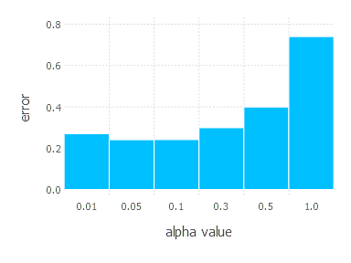
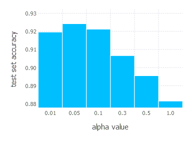
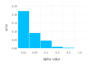
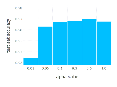
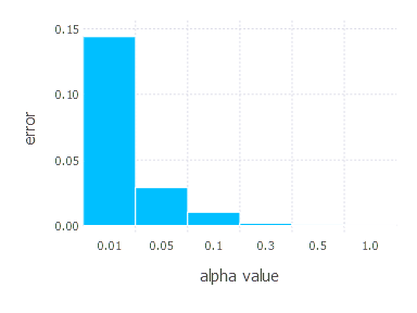
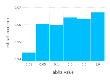
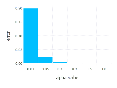
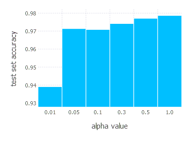
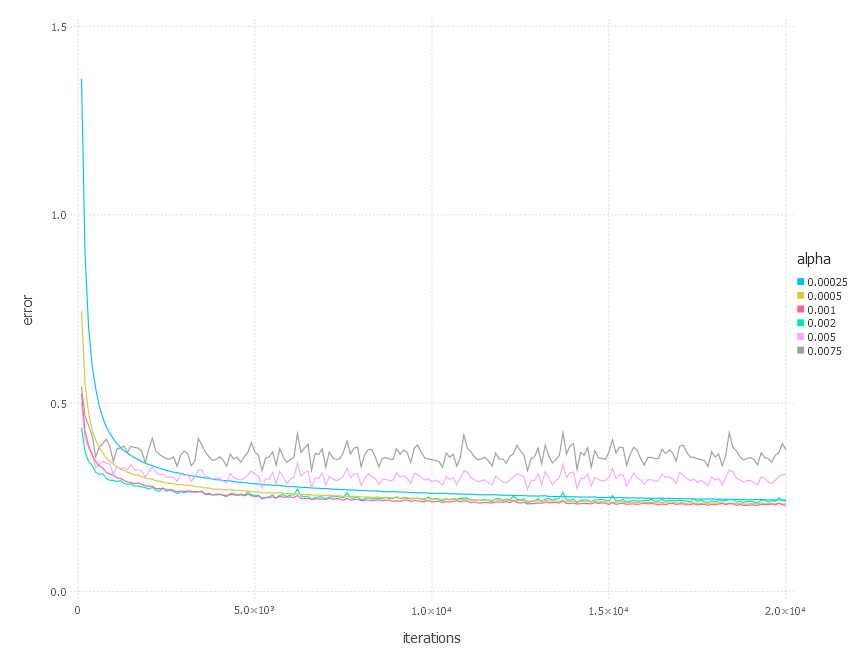
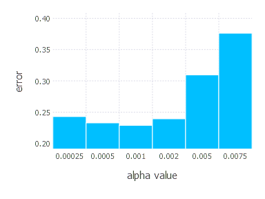
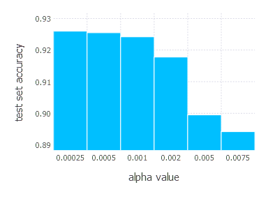
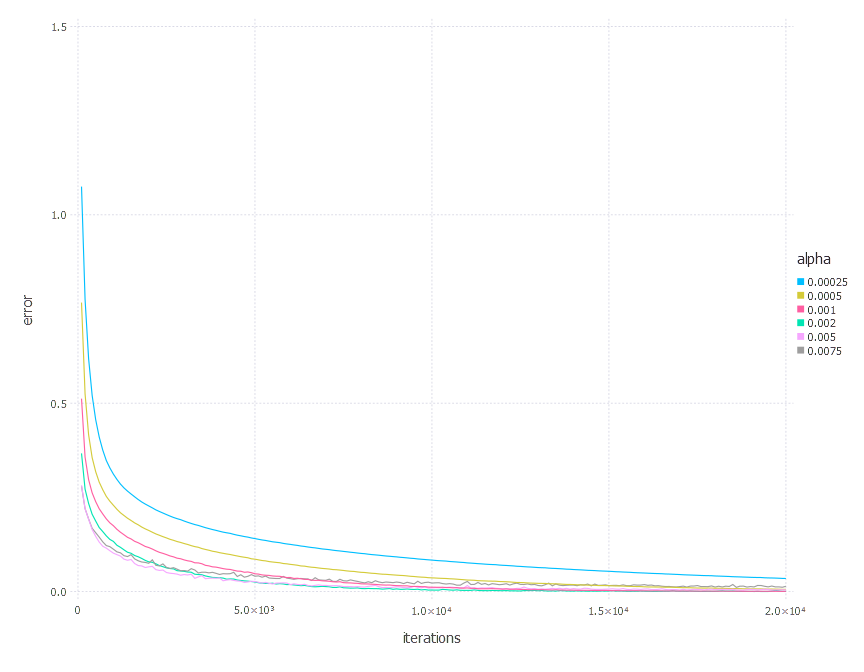
We will start this section by running experiments for one optimization technique at a time for various problems (all will be cross-entropy error function minimization for different neural network architectures with the problem of MNIST classification). The goal of these experiments is to find the best parameters’ set for given optimization technique - so for each of the algorithms and problems we will search through the parameter space - using a “brute force” approach (sometimes using “recommended default” values of parameters). We choose two basic evaluation metrics: error function value itself and test accuracy after 42 epochs (20000 iterations with mini batch size of 128). You should probably not stick too much to the test accuracy evaluation as non overfitting preventing routines were applied and so the results might suffer from it. Please consider test set accuracy as a sanity check rather than a mature proper evaluation metric.

Also, please be aware this is just a rough scan through the parameter space and final parametrization may not be the best one - it is just the best one we can find.

The second part of experiments will cover comparison of different techniques (using best parameters’ set for each technique and problem).

The set of problems, we will play with, includes:

• Network with linear layer and softmax output - also known as softmax classification
• Network with sigmoid layer (100 neurons), linear layer and softmax output
• Network with tanh layer (100 neurons), linear layer and softmax output
• Network with sigmoid layer (300 neurons), ReLU layer (100 neurons), sigmoid layer (50 neurons) again, linear layer and softmax output

For all optimization algorithms we will use mini-batch size of 128. We will run the algorithm for approx. 42 epochs (20000 iterations).

We will not include the code here directly as it would take most of this post content.

Stochastic Gradient Descent - experiments

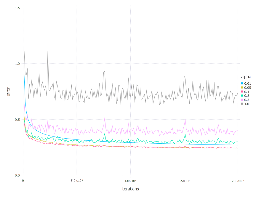
Momentum optimization algorithm involves learning rate \( \alpha \) parameter. Parameters we examined in these experiments are:

\[\alpha \in \{ 0.01, 0.05, 0.1, 0.3, 0.5, 1 \}\]

1. Network with linear layer and softmax output [SGD]

---

2. Network with sigmoid layer (100 neurons), linear layer and softmax output [SGD]

---

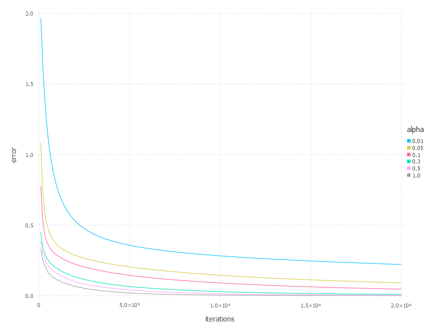
3. Network with tanh layer (100 neurons), linear layer and softmax output [SGD]

---

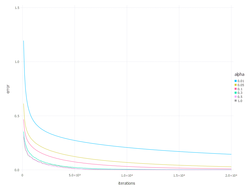
4. Network with sigmoid layer (300 neurons), ReLU layer (100 neurons), sigmoid layer (50 neurons) again, linear layer and softmax output [SGD]

---

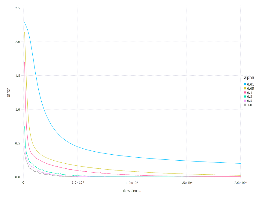
SGD Momentum - experiments

Momentum optimization algorithm involves two parameters - learning rate ( \alpha ) and momentum decay ( \gamma ). Parameters we examined in these experiments are:

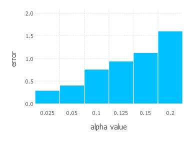
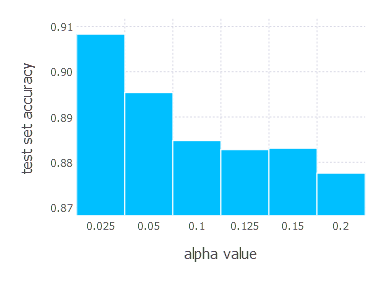
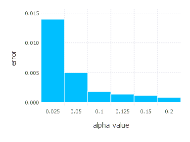
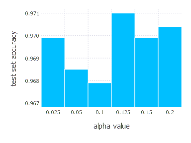
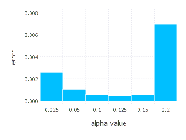
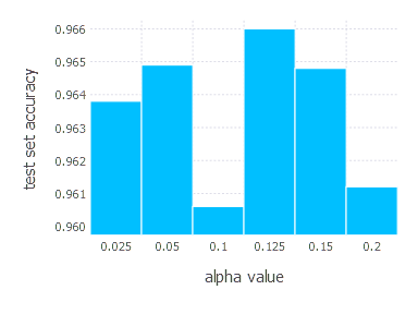
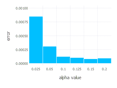
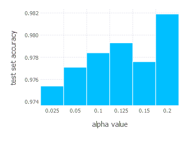
\[\alpha \in \{ 0.025, 0.05, 0.1 ,0.125, 0.15, 0.2 \} \quad \text{and} \quad \gamma = 0.9\]

---

1. Network with linear layer and softmax output [SGD Momentum]

---

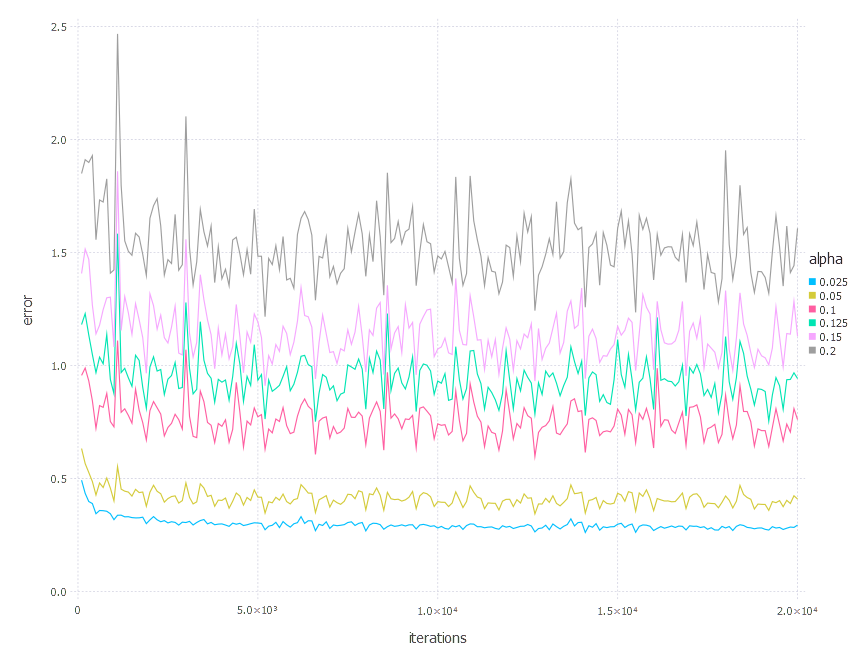
2. Network with sigmoid layer (100 neurons), linear layer and softmax output [SGD Momentum]

---

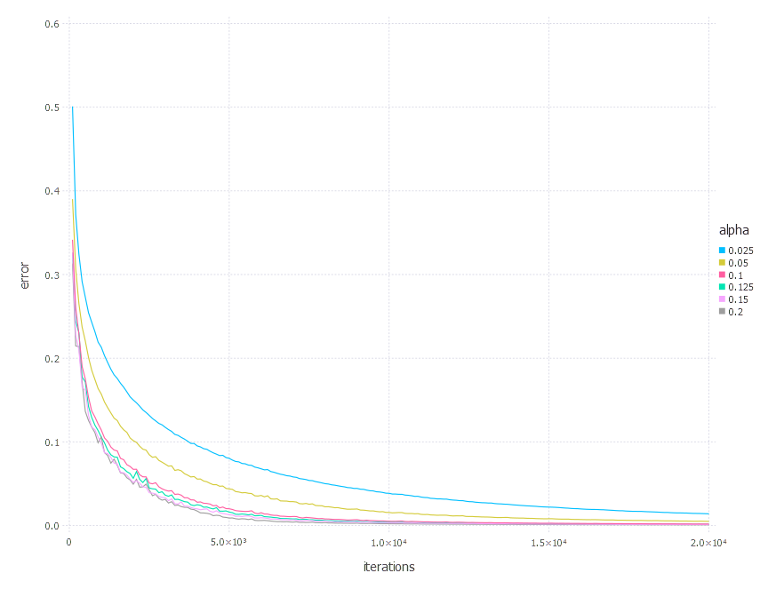
3. Network with tanh layer (100 neurons), linear layer and softmax output [SGD Momentum]

---

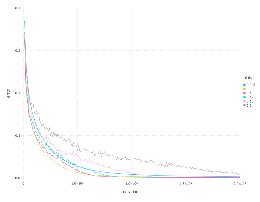
4. Network with sigmoid layer (300 neurons), ReLU layer (100 neurons), sigmoid layer (50 neurons) again, linear layer and softmax output [SGD Momentum]

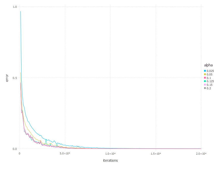
SGD Momentum - experiments

Momentum optimization algorithm involves two parameters - learning rate \(\alpha\) and momentum decay \(\gamma\). Parameters we examined in these experiments are:

\[\\ \alpha \in \{ 0.025, 0.05, 0.1, 0.125, 0.15, 0.2 \} \quad \text{and} \quad \gamma = 0.9 \\\]

1. Network with linear layer and softmax output [SGD Momentum]

2. Network with sigmoid layer (100 neurons), linear layer and softmax output [SGD Momentum]

3. Network with tanh layer (100 neurons), linear layer and softmax output [SGD Momentum]

4. Network with sigmoid layer (300 neurons), ReLU layer (100 neurons), sigmoid layer (50 neurons) again, linear layer and softmax output [SGD Momentum]

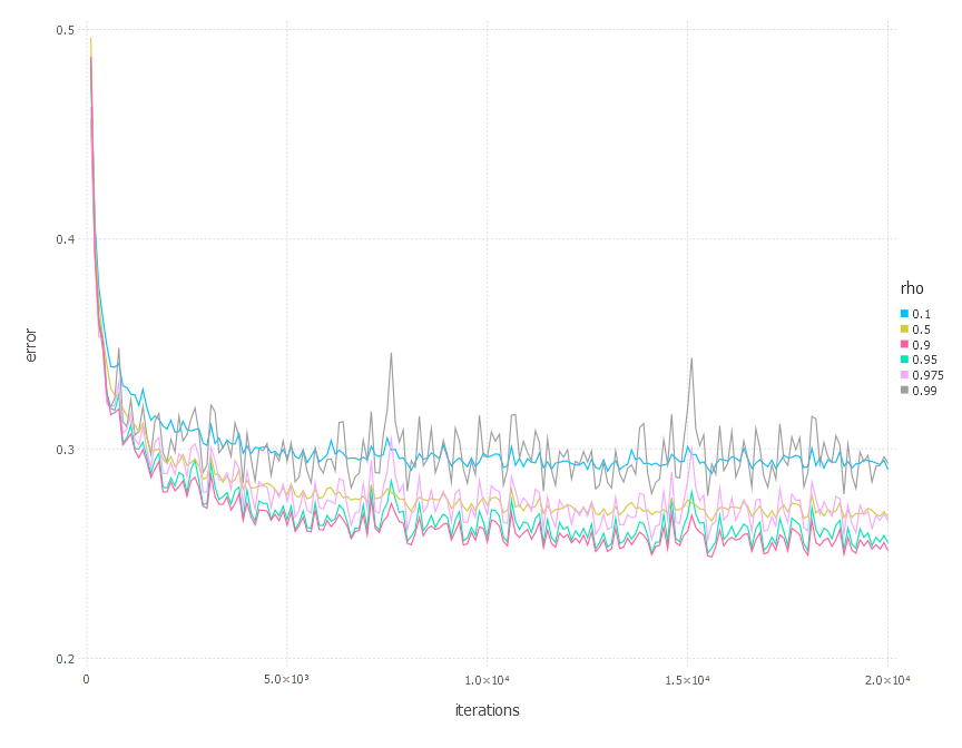
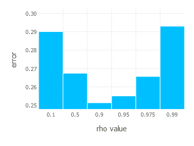
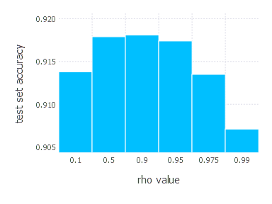
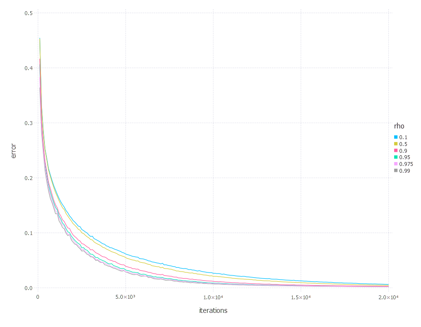
AdaDelta - experiments

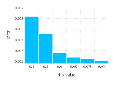
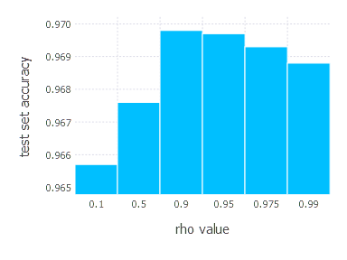
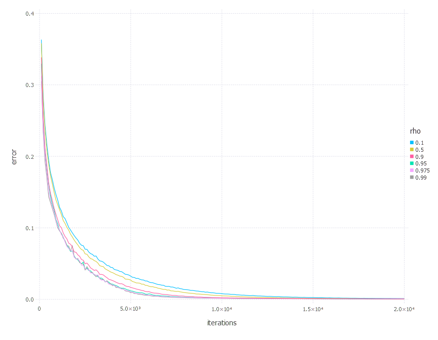
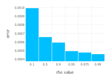
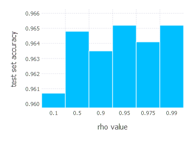
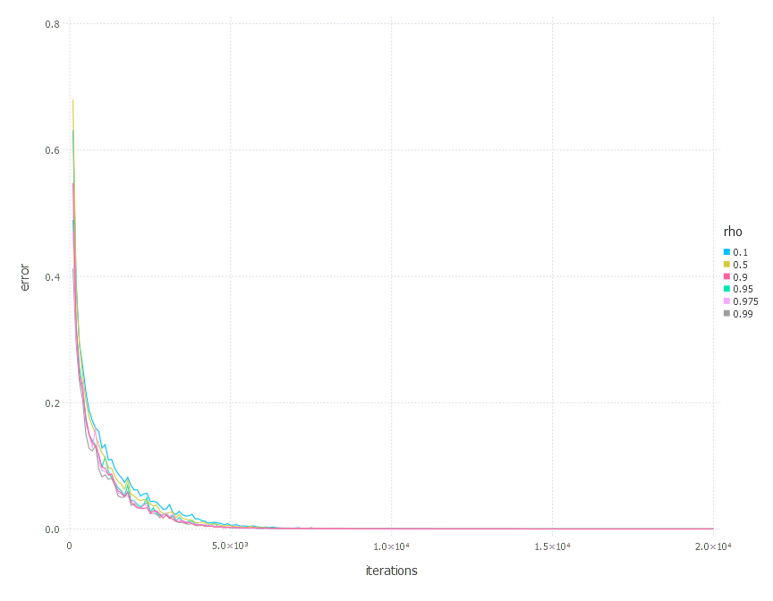
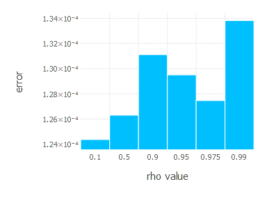
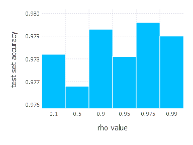
AdaDelta optimization algorithm involves one parameter - decay constant \(\rho\). Parameters we examined in these experiments are:

\[\rho\in \{ 0.1, 0.5, 0.9, 0.95, 0.975, 0.99 \}\]

1. Network with linear layer and softmax output [AdaDelta]

2. Network with sigmoid layer (100 neurons), linear layer and softmax output [AdaDelta]

3. Network with tanh layer (100 neurons), linear layer and softmax output [AdaDelta]

4. Network with sigmoid layer (300 neurons), ReLU layer (100 neurons), sigmoid layer (50 neurons) again, linear layer and softmax output [AdaDelta]

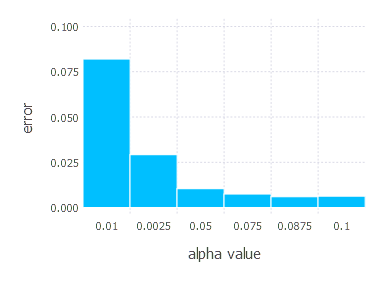
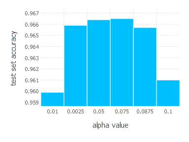
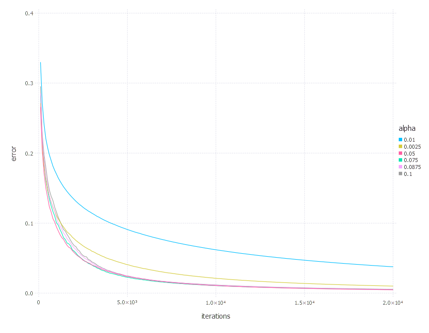
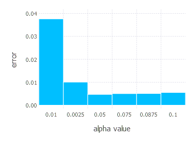
AdaGrad - experiments

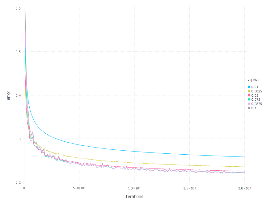
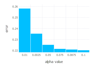
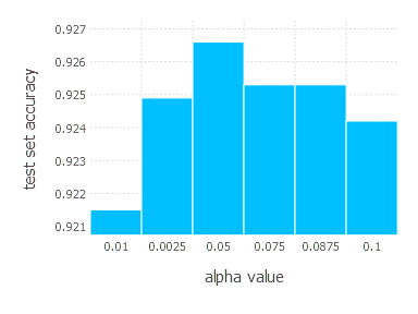
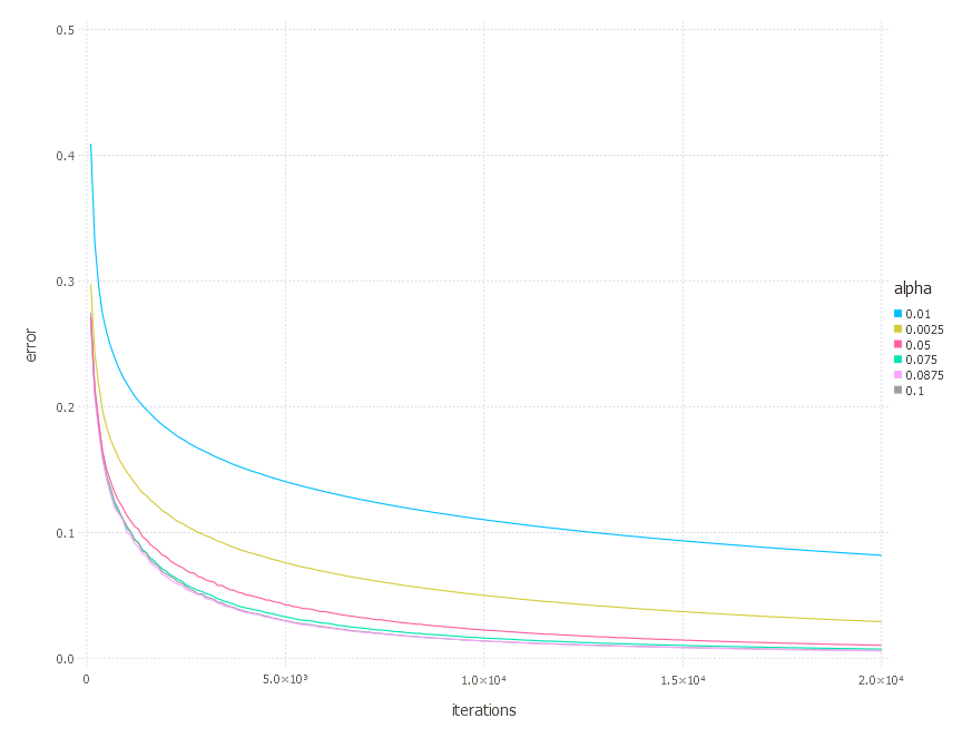
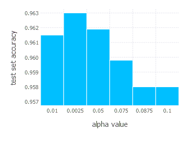
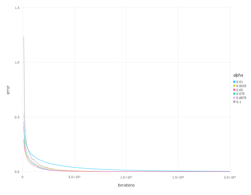
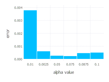
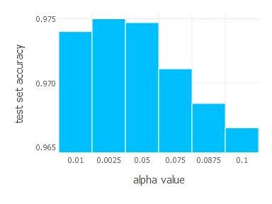
AdaGrad optimization algorithm involves one parameter - learning rate \(\alpha\). Parameters we examined in these experiments are:

\[\alpha \in \{ 0.01, 0.0025, 0.05, 0.075, 0.0875, 0.1 \}\]

1. Network with linear layer and softmax output [AdaGrad]

2. Network with sigmoid layer (100 neurons), linear layer and softmax output [AdaGrad]

3. Network with tanh layer (100 neurons), linear layer and softmax output [AdaGrad]

4. Network with sigmoid layer (300 neurons), ReLU layer (100 neurons), sigmoid layer (50 neurons) again, linear layer and softmax output [AdaGrad]

Adam - experiments

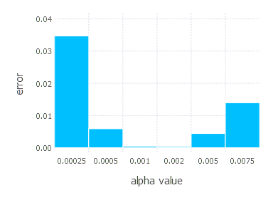
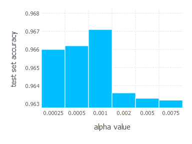
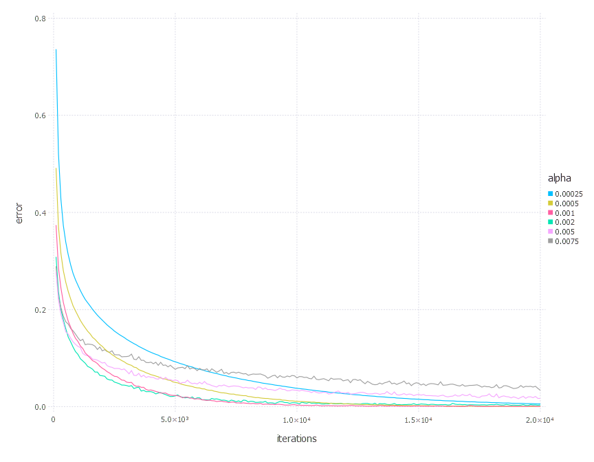
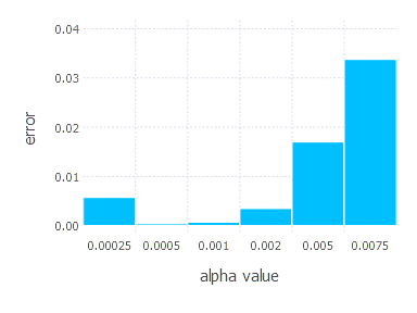
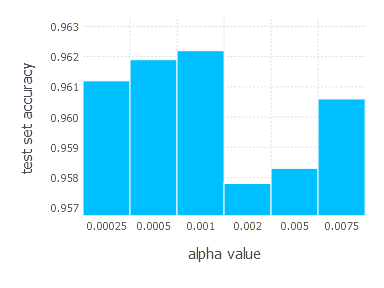
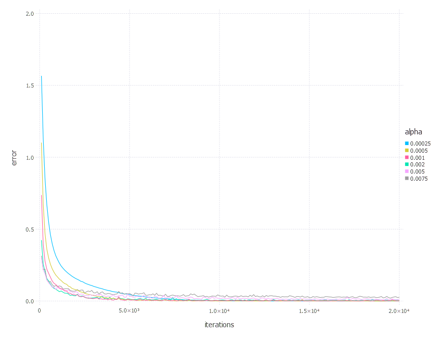
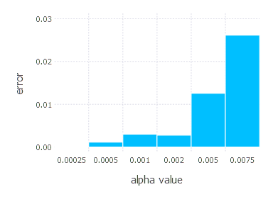
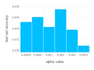
Adam optimization algorithm involves three main parameters, but here we set two of them \(\beta_1, \beta_2\) to default values proposed in the original paper \((\beta_1 = 0.9 \quad \beta_2 = 0.999)\). We only tweak learning rate \(\alpha\), examining in these experiments the following values:

\[\alpha \in \{ 0.00025, 0.0005, 0.001, 0.002, 0.005, 0.0075 \}\]

1. Network with linear layer and softmax output [Adam]

2. Network with sigmoid layer (100 neurons), linear layer and softmax output [Adam]

3. Network with tanh layer (100 neurons), linear layer and softmax output [Adam]

4. Network with sigmoid layer (300 neurons), ReLU layer (100 neurons), sigmoid layer (50 neurons) again, linear layer and softmax output [Adam]

Comparison of all methods

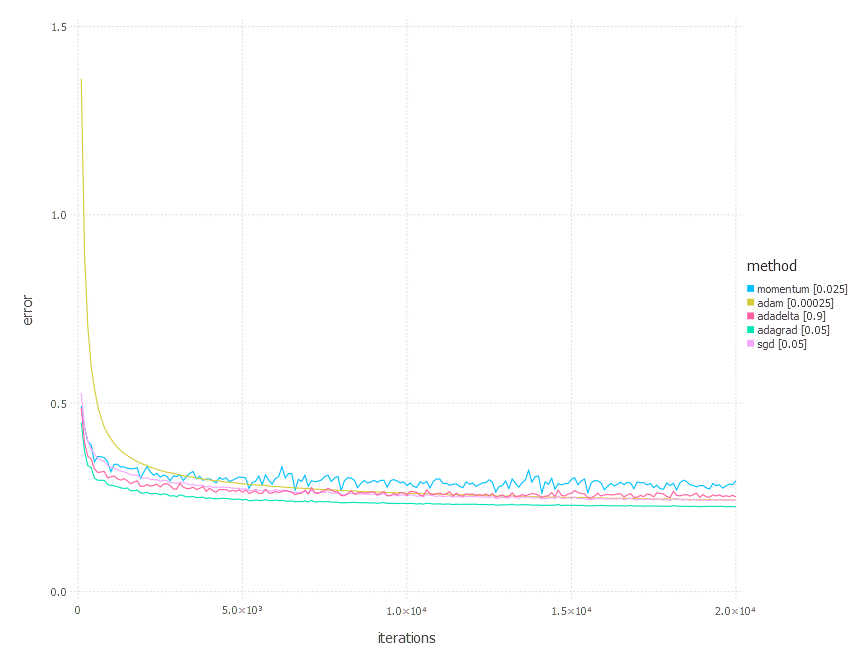
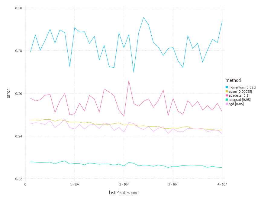
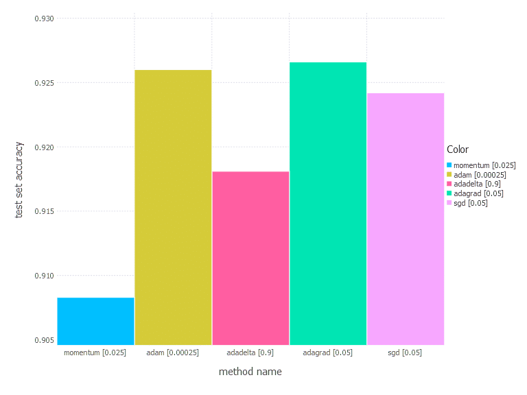
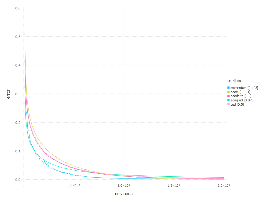
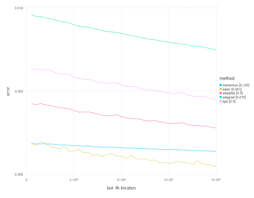
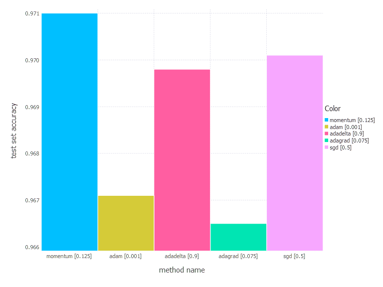
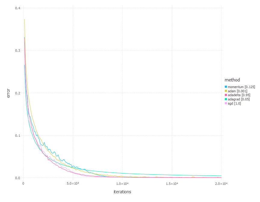
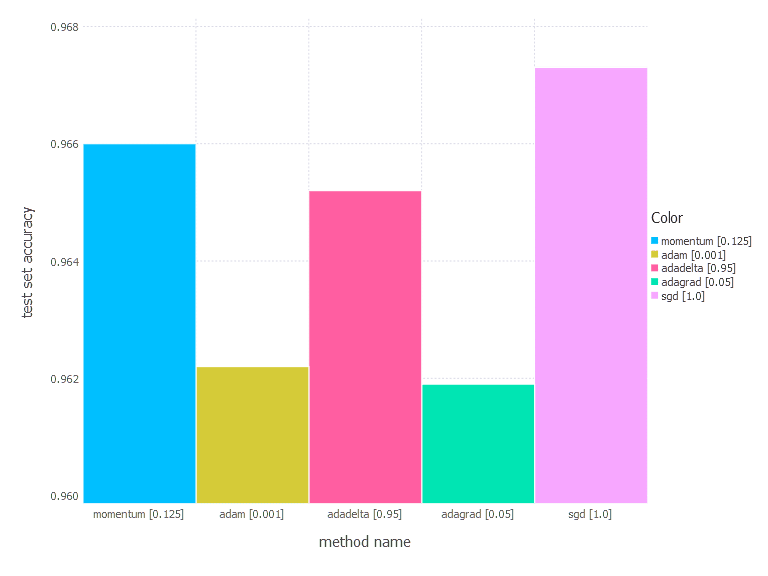
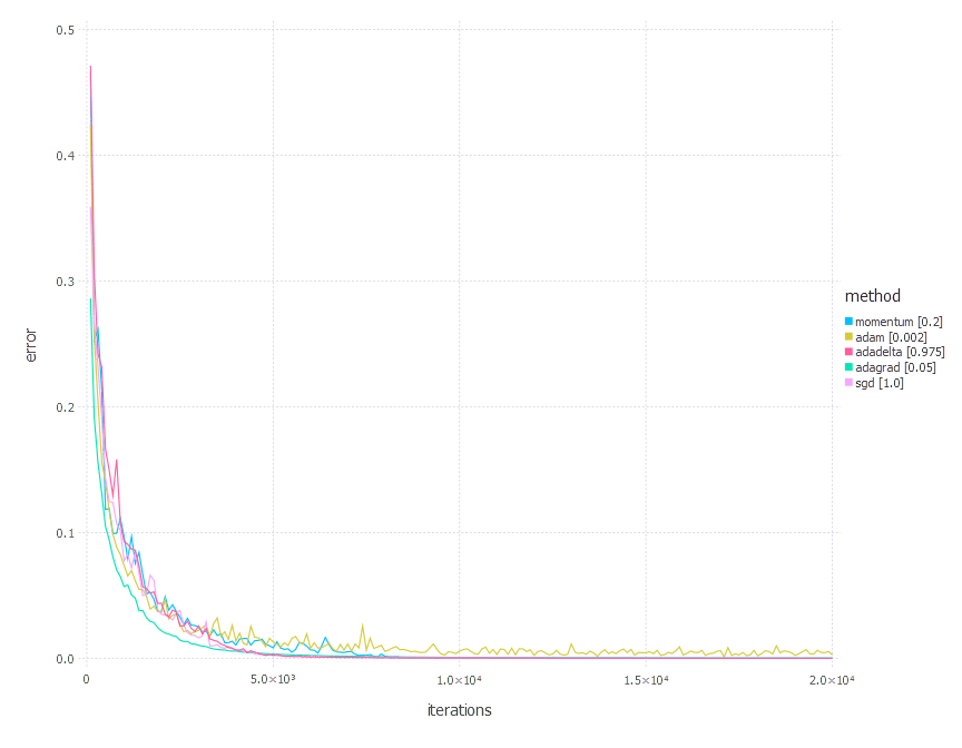
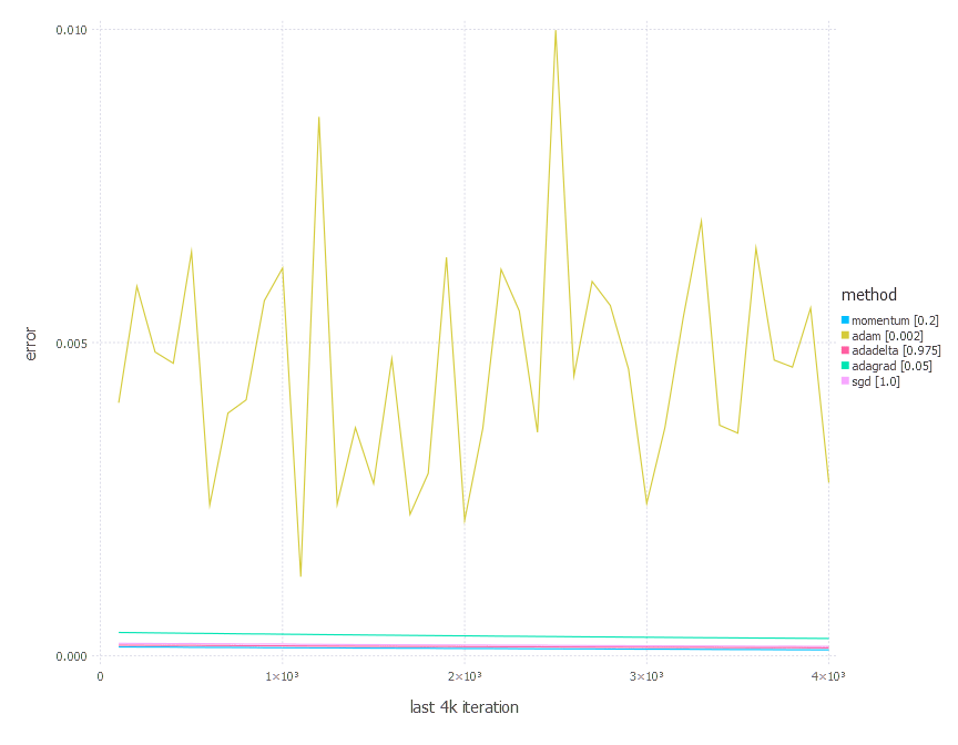
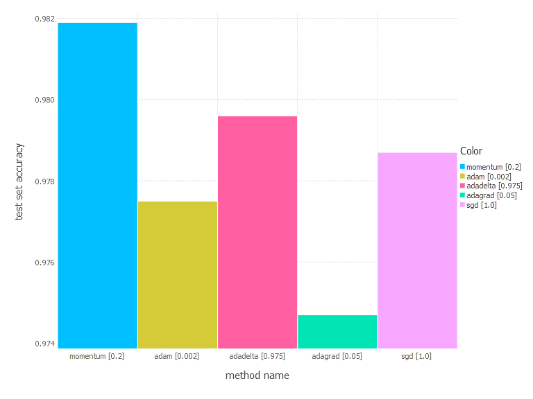
We will now present the comparison of all the methods described above. For each optimization technique, we will choose the parametrization that yields the best performance (in terms of error function value and test set accuracy) and compare the results for all 4 problems. For all problems, we will present charts showing error function value over time for each of the chosen methods, the last 4k iterations charts, and the final test set accuracy charts.

1. Network with linear layer and softmax output [Comparison]

2. Network with sigmoid layer (100 neurons), linear layer and softmax output [Comparison]

3. Network with tanh layer (100 neurons), linear layer and softmax output [Comparison]

4. Network with sigmoid layer (300 neurons), ReLU layer (100 neurons), sigmoid layer (50 neurons) again, linear layer and softmax output [Comparison]

Comments

From the results above, there is no one clear conclusion of which algorithm to choose and when. All of them perform differently depending on the problem and parametrization. AdaGrad is the best with the shallow problem (softmax classifier), AdaDelta is somewhere between all others—never leads, never fails badly too. Momentum and classical SGD seem to be a good fit for any problem of the above—they both produce leading results often. Adam has its big moment minimizing error of network #3 (with a bit worse accuracy there).

For all of the methods, the most challenging part is how to choose proper parameter values. And there is no clear rule for that too, unfortunately. The one ‘solid’ conclusion that can be drawn here is “to choose whatever works best for your problem”—I’m afraid. Although starting with simple methods—classical SGD or momentum—might be enough very often following what the experiments show.

Implementation-wise, optimization techniques presented here do not differ between one another that much too. Some of the algorithms expect a bit more computations and storage, but they all share the same linear complexity with respect to the number of parameters—choosing simpler methods might win another vote then.

What’s next?

The next step, we think is necessary to take, is to handle proper parameter initialization (now it is just a small random number centered at 0). Dealing with overfitting is a good way to go too. Overfitting prevention in neural networks may be realized in many different ways. L2 Regularization is the obvious choice, but there are alternative techniques like Dropout.

Among other interesting directions to move further, the one that is especially interesting is to check out convolutional neural networks—they open doors to many applications in image recognition tasks, and they are building blocks of generative models (GAN) for images. Another possible path is to investigate recurrent neural networks with great (by all rumors!) LSTM—as these let you handle the sequential data.

---