Large Scale Spectral Clustering with Landmark-Based Representation (in Julia)

Posted Jul 27, 2016 Updated Jan 19, 2025

By Kamil

8 min read

In this post we will implement and play with a clustering algorithm of a mysterious name Large Scale Spectral Clustering with Landmark-Based Representation (or shortly LSC – corresponding paper here). We will first explain the algorithm step by step and then map it to Julia code (github link).

Spectral Clustering

Spectral clustering (wikipedia entry) is a term that refers to many different clustering techniques. The core of the algorithm does not differ though. In essence, it is a method that relies on spectrum (eigendecomposition) of input data similarity matrix (or its transformations). Given input dataset encoded in a matrix $X$ (such that each single data entry is a column of that matrix) – spectral clustering requires a similarity (adjacency in case of graphical interpretation) matrix $A$ where

A_{i j} = f (X_{\cdot i}, X_{\cdot j})

and function $f$ is some measure of similarity between data points.

One specific spectral clustering algorithm (Ng, Jordan, and Weiss 2001) relies on matrix $W$ given by

W = D^{- 1 / 2} A D^{- 1 / 2}

where $D$ is a diagonal matrix with diagonal elements $(i, i)$ corresponding to sum of $i$ -th row of $A$ .

In Jordan, Weiss algorithm first $k$ (with largest eigenvalue) eigenvectors of $W$ are computed and (after normalization) they go as input to k-means to produce final dataset partition (clustering). Same idea motivates authors of LSC. The core idea of the LSC method is to limit the complexity of EVD of $W$ .

Large Scale Spectral Clustering with Landmark-Based Representation

One possible way to go to limit EVD complexity is to reduce the original problem to another (easier) one. In LSC paper authors construct matrix similar to $W = D^{- 1 / 2} A D^{- 1 / 2}$ in a clever way. Matrix $W$ used in LSC has the following form:

W = {\hat{Z}}^{T} \hat{Z}

(authors construct $\hat{Z}$ such that it is sparse matrix of dimensionality much lower than original matrix)

Therefore it is sufficient enough to compute Singular Value Decomposition of sparse small matrix $\hat{Z}$ instead of computing EVD of $W$ . Please recall, SVD of any matrix $X$ produces eigenvectors of both $X X^{T}$ and $X^{T} X$

Construction of matrix $\hat{Z}$

Matrix $\hat{Z}$ is defined as:

\hat{Z} = D^{- 1 / 2} Z

where $Z$ is a sparse matrix that can be seen as new input data $X$ representation and again $D^{- 1 / 2}$ is diagonal matrix with row sums entries of $Z$ . Columns of matrix $Z$ are defined as coefficients of a weighted sum (linear combination) of a centroid vectors given by prior k-means clustering (or randomly chosen input vectors!). These vectors are called Landmarks

Here is exact routine to get matrix $Z$ (assuming choice based on k-means) :

Given input data matrix $X$ compute $p$ k-means centroids of $X$ and store them in $U$
For each data point $x_{i}$ produce sparse vector $z_{i}$ with non zero entries corresponding to the closest $r$ clustering centroids from $U$ given by gaussian kernel
Normalize $z_{i}$ and store in matrix $Z$ as an $i$ -th column

Computing eigenvectors of matrix $W$ – spectral clustering core part

Having $W$ constructed according to aforementioned formulas, the next core part of the algorithm is to compute EVD of $W$ . As was mentioned, eigendecomposition is not computed directly on $W$ as this would be inefficient. Instead of direct EVD on $W$ SVD of sparse and smaller $\hat{Z}$ is computed. SVD of $\hat{Z}$ is given by:

\hat{Z} = A Σ B^{T}

(note that it is of course different $A$ than similarity matrix above)

Here authors compute matrix $A$ from SVD fast to finally compute $B$ according to the formula:

B^{T} = Σ^{- 1} A^{T} \hat{Z}

Matrix $B$ contains our final eigenvectors that are input for final k-means clustering. (our implementation skips that as svd routine in Julia computes $B$ directly).

Final step: k-means on eigenvectors

Now having eigenvectors of $W$ authors apply classical k-means algorithm to get final data clustering. The main gain here is the computational complexity reduction. Normally, eigendecomposition has complexity of $O (n^{3})$ in data set cardinality $n$ . After a bit of gymnastics as above they achieve $O (p^{3} + p^{2} n)$ where $p$ is number of centroids from initial k-means (or number of randomly selected landmarks in case of such algorithm variant)

LSC – implementation

Let’s start with routine to get $p$ landmarks.

        
      
using Clustering;
using Distances;

function getLandmarks(X, p, method=:Random)
    if(method == :Random)
        numberOfPoints = size(X,2);
        landmarks = X[:,randperm(numberOfPoints)[1:p]];
        return landmarks;
    end

    if(method == :Kmeans)
        kmeansResult = kmeans(X,p)
        return kmeansResult.centers;
    end

    throw(ArgumentError('method can only be :Kmeans or :Random'));
end

We also need a function to compute $\hat{Z}$

        
      
function gaussianKernel(distance, bandwidth)
    exp(-distance / (2*bandwidth^2));
end


function composeSparseZHatMatrix(X, landmarks, bandwidth, r)

    distances = pairwise(Distances.Euclidean(), landmarks, X);
    similarities = map(x -> gaussianKernel(x, bandwidth), distances);
    ZHat = zeros(size(similarities));

    for i in 1:(size(similarities,2))
        topLandMarksIndices = selectperm(similarities[:,i], 1:r, rev=true);
        topLandMarksCoefficients = similarities[topLandMarksIndices, i];
        topLandMarksCoefficients = topLandMarksCoefficients / sum(topLandMarksCoefficients);
        ZHat[topLandMarksIndices,i] = topLandMarksCoefficients;
    end
    return diagm(sum(ZHat,2)[:])^(-1/2) * ZHat;

end

Finally, we can implement core LSC routine as

        
      
function LSCClustering(X, nrOfClusters, nrOfLandmarks, method, nonZeroLandmarkWeights, bandwidth)
    landmarks = getLandmarks(X, nrOfLandmarks, method)
    ZHat = composeSparseZHatMatrix(X, landmarks, bandwidth, nonZeroLandmarkWeights)
    svdResult = svd(transpose(ZHat))
    clusteringResult = kmeans(transpose(svdResult[1])[:1:nrOfClusters],nrOfClusters);
    return clusteringResult
end

Please note that our implementation differs a bit from the original one (here, we consider first $k$ eigenvectors as new data representation).

LSC - toy data examples

Here is the result of LSC clustering (with k-means landmark generation) on toy datasets - they all have cardinality 2000
(Datasets are available to download: cassini, shapes, smiley and spirals)

        
      
using Gadfly 
# smiley example
smiley = readtable("smiley.csv");
smiley = transpose(convert(Array{Float64,2}, smiley[:,1:2]))
result = LSCClustering(smiley, 4, 50, :Kmeans, 4, 0.4)
plot(x = smiley[1,:], y = smiley[2,:], color = result.assignments)

# spirals example
spirals = readtable("spirals.csv");
spirals = transpose(convert(Array{Float64,2}, spirals[:,1:2]))
result = LSCClustering(spirals, 2, 150, :Kmeans, 4, 0.04)
plot(x = spirals[1,:], y = spirals[2,:], color = result.assignments)

# shapes example
shapes = readtable("shapes.csv");
shapes = transpose(convert(Array{Float64,2}, shapes[:,1:2]))
result = LSCClustering(shapes, 4, 50, :Kmeans, 4, 0.04)
plot(x = shapes[1,:], y = shapes[2,:], color = result.assignments)

# cassini example
cassini = readtable("cassini.csv");
cassini = transpose(convert(Array{Float64,2}, cassini[:,2:3]))
result = LSCClustering(cassini, 3, 50, :Kmeans, 4, 0.4)
plot(x = cassini[1,:], y = cassini[2,:], color = result.assignments)

Obviously, even though results look quite promising we cannot pass over one problem: parameter choice. Here, we have quite a few of them - number of landmarks, $Z$ density (via $r$ ), and Gaussian bandwidth - and sometimes (this time in particular!) choosing working set of parameters is not an easy task.

LSC - MNIST dataset

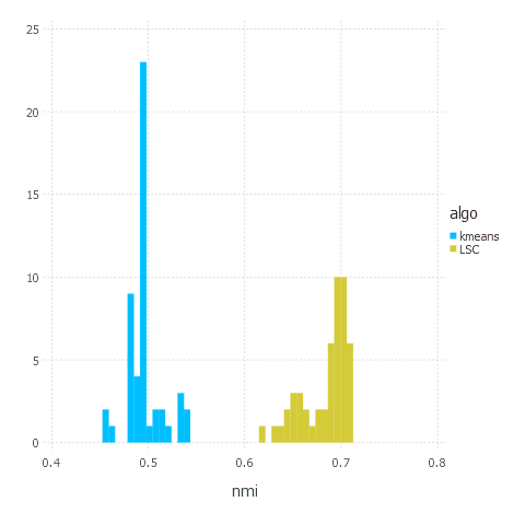
Let’s finally try LSC on a ‘more serious’ dataset - handwritten digits dataset called MNIST. In this experiment we are going to compare LSC with classical k-means. We are going to use NMI (normalized mutual information) clustering quality as our metric.

Let’s quickly implement NMI (according to this)

        
      
# Pkg.add("Iterators")
using Iterators
 
function entropy(partitionSet, N)
    return mapreduce(x -> -(length(x) / N) * log(length(x) / N), +, partitionSet)
end

function getPartitionSet(vector, nrOfClusters)
    d = Dict(zip(1:nrOfClusters,[Int[] for _ in 1:nrOfClusters]));
    for i in 1:length(vector)
        push!(d[vector[i]], i)
    end
    return collect(values(d))
end


function mutualInformation(partitionSetA, partitionSetB, N)


    anonFunc = (x) -> (
                intersection = size(intersect(partitionSetA[x[1]], partitionSetB[x[2]]),1);
                return intersection > 0 ?
                        (intersection/N) * log((intersection * N) / (size(partitionSetA[x[1]],1) * size(partitionSetB[x[2]],1))) : 0;
    )

    mapreduce(anonFunc, + , product(1:length(partitionSetA),1:length(partitionSetB)))
end


function normalizedMutualInformation(partitionSetA, partitionSetB, N)
    mutualInformation(partitionSetA, partitionSetB, N) / ((entropy(partitionSetA, N)  + entropy(partitionSetB, N)) / 2)
end

And now we are ready to go. Let’s compare our results with k-means for a sanity check (running 50 experiments):

        
      
# Pkg.add("MNIST")
using MNIST;
# reading dataset (60k objects)
data, labels = MNIST.traindata(); # using testdata() instead will return smaller (10k objects) dataset 
# normalizing it 
data  = (data .- mean(data,2)) / std(data .- mean(data,2));

nrOfExperiments = 50; 
kmeansResults = [];
LSCResults = [];
for i in 1:nrOfExperiments
   LSCMnistResult = LSCClustering(data, 10, 350, :Kmeans, 5, 0.5);
   kmeansMnistResult = kmeans(data,10);

   kmeansNMI = normalizedMutualInformation(getPartitionSet(kmeansMnistResult.assignments, 10) , getPartitionSet(labels + 1 ,10), 60000)
   LSCNMI = normalizedMutualInformation(getPartitionSet(LSCMnistResult.assignments, 10) , getPartitionSet(labels + 1 ,10), 60000)
   push!(kmeansResults, kmeansNMI);
   push!(LSCResults, LSCNMI);

end

# Pkg.add("DataFrames");
# Pkg.add("Gadfly");
using DataFrames; 
using Gadfly; 

df = DataFrame(nmi = [kmeansResults; LSCResults], algo = [["kmeans" for _ in 1:50];["LSC" for _ in 1:50]]);
plot(df, x="nmi",  color="algo", Geom.histogram(bincount=40));

Summary

That’s it. LSC clustering algorithm turned out to be better in terms of quality (as promised in a paper) than k-means. The main challenge though was proper parameters’ values choice - usually we had to tweak Gaussian kernel bandwidth and number of landmarks a bit to make the algorithm produce good results. K-means does not suffer from that problem so it is usually ‘practically’ faster - as you don’t need to experiment with parameters (which is a hard problem itself) to get good clustering.

Clustering

This post is licensed under CC BY 4.0 by the author.