Counterfactual Regret Minimization - the core of Poker AI beating professional players
The last 10 years have been full of unexpected advances in artificial intelligence. Among great improvements in image processing and speech recognition - the thing that got lots of media attention was AI winning against humans in various kinds of games. With OpenAI playing Dota2 and DeepMind playing Atari games in the background, the most significant achievement was AlphaGo beating Korean master in Go. It was the first time a machine presented super-human performance in Go marking - next to DeepBlue-Kasparov chess game in 1997 - a historical moment in the field of AI.
Around the same time, a group of researchers from USA, Canada, Czech Republic, and Finland had been already working on another game to solve: Heads Up No Limit Texas Hold’em
The very first big success was reported in 2015 when Oskari Tammelin, Neil Burch, Michael Johanson, and Michael Bowling created a computer program called Cepheus - AI playing Heads Up Limit Texas Hold’em. They published their work in papers with straightforward titles: Solving Heads-Up Limit Texas Hold’em* and Heads-up Limit Hold’em Poker is Solved
Cepheus - AI playing Limit Texas Hold’em Poker
Even though the titles of the papers claim solving poker - formally it was essentially solved. Essentially solving Heads Up Limit* Texas Hold’em meant researchers were able to come up with an approximation (indistinguishable from the original one for a human during a lifetime) of a strategy profile called Nash Equilibrium. In two-person zero-sum games, playing a strategy from a Nash Equilibrium is also the best any player can do in case of no knowledge of his opponent’s strategy (please take a look below for more details on basics of game theory).
(image from http://poker.srv.ualberta.ca/)
Note:
The main difference between limit and no-limit versions is the branching factor. In limit Texas Hold’em, there is a limit on the number and size of the bets, and so the number of actions in a given situation is limited for both players. In no-limit Texas Hold’em, there is no such limitation. Limit HUTH game size (number of decision points) is estimated to around \(10^{14}\) while its no-limit version size goes to around \(10^{160}\). It makes solving the no-limit version of HUTH a much more difficult task. A big success in limit Texas Hold’em poker was therefore still far away to be repeated for its no-limit version.
Essentially, researchers working on Cepheus computed all possible responses for any possible game situation offline efficiently. Terabytes of vectors representing probability distributions over possible actions in all game situations were computed and stored. While this does not sound as sexy as AlphaGo’s deep neural network, the algorithm for computing Nash Equilibrium strategy profile is to some extent similar to the one used in AlphaGo/AlphaZero. The common thing for both solutions is learning from playing against itself. The Cepheus’ core algorithm - Counterfactual Regret Minimization - is also the main subject of this post.
DeepStack - Neural Network-based AI playing Heads Up No-Limit Texas Hold’em
Around 2 years after Cepheus, another successful poker bot was revealed - this time it could win against humans in the no-limit version of Heads Up Texas Hold’em. Its name was DeepStack, and it used continual re-solving aided by neural networks as a core.
Re-solving is one of the subgame solving techniques. A subgame is a game tree rooted in the current decision point. From the very high-level view, then subgame solving means solving a subgame in separation from the parent nodes. In other words, re-solving is a technique to reconstruct a strategy profile for only the remainder of the game at the given decision point.
Creators of DeepStack used continual re-solving where only two vectors were maintained throughout the game. The two vectors turned out to be sufficient to continuously reconstruct a strategy profile that approximates Nash Equilibrium in a current subgame (decision point).
In DeepStack, a deep neural network was used to overcome computational complexity related to continual re-solving proposed by its creators. This complexity issue comes from counterfactual values vector re-computation in any decision point throughout the game. A straightforward approach is to apply a Counterfactual Regret Minimization solver, but this is practically infeasible. DeepStack handles this by limiting both depth and breadth (this is somehow similar to AlphaGo’s value and policy networks) of the CFR solver. Breadth is limited by action abstraction (only fold, call, 2 or 3 bet actions, and all-in are valid), while depth is limited by using a value function (estimated with deep neural network) at a certain depth of the counterfactual value computing procedure.
To evaluate DeepStack’s performance against humans, 33 professional players from 17 countries were selected (with the help of International Federation of Poker) to play 3000 hands each. Games were performed via an online interface. DeepStack noted an average win of 492 mbb/g (meaning it could win 49 big blinds per 100 hands dealt). DeepStack won against all of the players except one for whom the result was not statistically significant.
This was the first time a machine could compete with humans in the No-Limit version of Heads Up Texas Hold’em Poker*
Note:
To be perfectly correct: DeepStack and Libratus (described below) were both created around the same time. DeepStack creators organized the match first, so they may be considered as those who could compete with humans first. But the concepts and ideas on how to build both systems emerged around the same time. Also, the skill range of opponents for DeepStack and Libratus was different - DeepStack’s opponents were considered weaker, especially in heads-up games.
Some DeepStack games are available on DeepStack’s YouTube channel.
DeepStack hits a straight on a river, goes all in against human having a flush.
An example of DeepStack (sort of) bluffing on a turn forcing human to fold.
Libratus - DeepStack’s main rival from Carnegie Mellon University
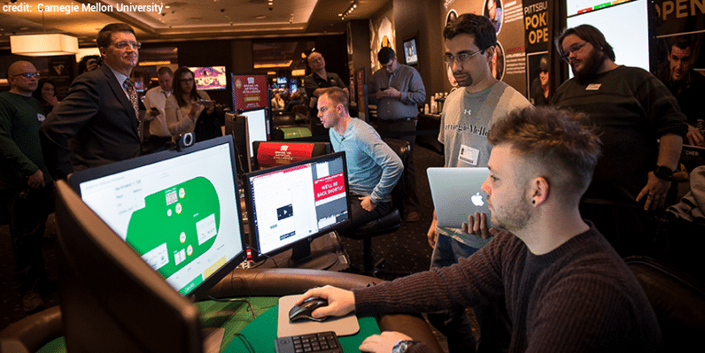
In January 2017, another step towards superhuman poker performance was made. Libratus - AI playing Heads Up No-Limit Texas Hold’em developed by Tuomas W. Sandholm and his colleagues from Carnegie Mellon University - defeated a team of 4 professional players: Jason Les, Dong Kim, Daniel McCauley, and Jimmy Chou. The event - Brains vs AI - took place in a casino in Pittsburgh, lasted 20 days, and resulted in around 120,000 hands being played. The participants were considered to be stronger than DeepStack’s opponents. The prize pool of 200k USD was divided among all 4 players proportionally to their performance. Libratus was able to win individually against all of the players, beating all players 147 mbb/g on average.
A mix of three main different methods was used in Libratus:
-
Blueprint strategy computed with Monte Carlo Counterfactual Regret Minimization
The blueprint strategy is a pre-computed strategy of the abstraction of the game (abstraction is a smaller version of the game where actions and cards are clustered to reduce game size) that serves as a reference for other components of the system. The blueprint for the first two rounds is designed to be dense (meaning action abstraction includes more different bet sizes). Libratus plays according to the blueprint strategy at the beginning of the game and then switches to nested subgame solving for decision points deeper in the game tree.
-
Nested subgame solving
Given a blueprint strategy and a decision point in a game, Libratus’s creators applied a novel subgame solving technique - nested subgame solving. Subgame solving techniques produce reconstructed strategy for the remaining of the game - in practice, better than the blueprint reference strategy. The details of this technique are described in a paper chosen to be the best one from NIPS 2017.
-
Self-improvement during the event
Opponents’ actions (bet sizes) were recorded during the event to extend the blueprint strategy after each day. Frequent bets that had been far away from current action abstraction (those that could potentially exploit Libratus the most) were added to the blueprint during nights between event days.
In December 2017, authors of the Nested Subgame Solving paper, Tuomas Sandholm and Noam Brown, held an AMA on r/machinelearning. Among many questions asked, there is one about comparison of DeepStack and Libratus.
All the poker programs presented so far used some form of Counterfactual Regret Minimization as their core component. In Cepheus, its fast variant was used to pre-compute Nash equilibrium offline; DeepStack used a CFR-like algorithm (aided by neural networks) for subgame solving; and finally in Libratus, the blueprint strategy (Nash Equilibrium of a game abstraction) was computed with Monte Carlo counterfactual regret minimization.
The goal of the rest of this post is to present basic bits required to understand Counterfactual Regret Minimization. To get there, we will go through basics of game theory first. This will give us an understanding of what we are looking for: what a strategy profile is and why Nash Equilibrium is a good one in poker. Once we have that knowledge, we will go to another interesting topic: no-regret learning. One simple framework called ‘combining expert advice’ will turn out to be the core of CFR.
Basics of game theory
Game theory is a field of mathematics providing handy tools for modeling and reasoning about interactive situations. These interactive situations called games may have very different nature depending on many factors like the number of players, structure of utilities, moves order, and many more. Based on these characteristics, we can classify games into types. Once we classify a game, we can start reasoning about it using known generic theorems that hold for our game type. In this post, we will focus on Heads Up No-Limit Texas Hold’em Poker. Let’s then first find out how game theory classifies our game so we can use proper tools later.
What type of game is Heads Up NLTH poker?
HU NLTH is an example of a two-person zero-sum finite game with imperfect information and chance moves.
Let’s dismantle this into pieces:
- Two-person because there are two players involved.
- Game being finite implies there is a finite number of possible histories of actions. In poker, this number is enormous but indeed finite.
- Game is considered zero-sum if all payoffs (players’ gains/losses) sum up to zero. This holds for poker. Unless there is a draw where no player wins anything, the pot goes to one of the players, making the other one lose the equivalent (rakes are omitted).
- Imperfect information game means players are not aware of the exact state of the game – there is hidden information that players are not aware of. In poker, this hidden information is the opponent’s hand.
- Game with chance moves means there are some random elements of the game players have no control over – in poker, these are consecutive random betting rounds or initial cards dealing.
All of these will imply certain theorems/models that we will have a right to use on our way to understand CFR.
What does it mean to have a strategy in a Heads Up NLTH poker game?
Loosely speaking, a strategy describes how to act in every single possible situation. It is a recipe for how to act in the entire game, a lookup table you can read your actions from.
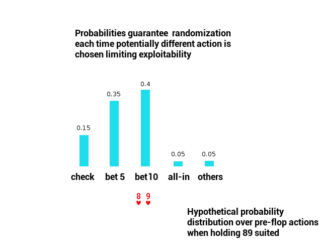
In games like poker, actions chosen via strategies cannot be fully deterministic. Randomization is necessary – if players didn’t do it, their betting pattern would be quickly learned and exploited. In game theory, randomization of decisions in decision points is realized via probabilities.
Behavioral strategy is a set of probability distributions over actions in decision points. It is a full description of how to act (hence the name) in all game situations. In a single game playout, exact actions are drawn from probability distributions associated with decision points.
A strategy profile, on the other hand, is a set of strategies for all players involved in a game. In our Heads Up NLTH poker scenario, the strategy profile consists of two strategies (one for each player).
Given a strategy profile, we can already emulate playing poker between players. A single game play would be a sequence of actions drawn from probability distributions given by players’ strategies (+ dealer actions as chance). Once a game play is over, players gain their utilities (or payoffs).
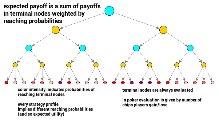
Because we are set up in a probabilistic framework, we can consider expected utilities for players. Every strategy profile then directly indicates expected utilities (expected payoffs) for both players. It means we can evaluate strategies and strategy profiles via expected utilities.
Why Nash Equilibrium?
Our main algorithm – CFR – produces an approximation of a strategy profile called Nash Equilibrium.
Nash Equilibrium is a strategy profile (set of strategies for all players involved) such that no single player has an incentive to deviate. It represents a balance between players, a point where no player gains from changing his/her strategy. We say both players play a Nash Equilibrium strategy profile if changing one player’s strategy does not bring any additional value (in terms of utility) when the other player plays his original strategy (he does not change it) – both players play best responses to one another.
A few questions about Nash Equilibrium arise. First, does Nash Equilibrium exist for poker in the first place? If it does, is there only one or more NE? Which one will be computed by CFR? Are we guaranteed to land on the best NE?
The first question about NE existence can be addressed via Nash’s Existence Theorem stating that for finite games (that includes poker), Nash Equilibrium is guaranteed to exist*.
Note:
To be precise, it proves mixed strategy NE existence, but this is equivalent to the existence of behavioral strategy NE.
Another important piece is the Minimax Theorem, proving that for two-player zero-sum finite games, there exists the best single possible utility called value of the game both players in equilibrium gain.
It is then also true that all Nash Equilibria values in poker are equal – they produce the same expected utility. Even more, they are interchangeable: you can play any strategy against any opponent strategy from any Nash Equilibrium, and you will land with the same payoff – value of the game. That again holds for all zero-sum two-player games.
Moreover, even though the value of the game in poker may not be zero (is there an ‘advantage symmetry’ between dealer position and blinds inequality?), in the long run, it will vanish to zero because in Heads Up NLTH poker, the dealer button moves from one player to another between rounds, playing Nash Equilibrium will in practice result in zero payoff then (you will not lose playing it in expectation). Exploitability of a strategy from a Nash Equilibrium pair is zero – it means that if you play it, your opponent’s best exploit strategy will have a zero payoff in expectation. You are guaranteed to draw in the worst case.
If you choose to play any strategy from any Nash Equilibrium, you are guaranteed not to lose. In practice, though, since it is highly unlikely your human opponent plays it, you will outperform him in expectation because he will be deviating from his NE strategy and so he will get lower payoff. And because the game of poker is a two-player zero-sum game, it equivalently means you will get higher payoff. In practice, then, playing Nash Equilibrium wins in expectation (against mistake-prone humans).
Nash Equilibrium exists, and there is no difference which one CFR computes. As long as it computes one, playing it guarantees not to lose in expectation.
How does a poker game tree look like?
One very convenient way of representing games such as poker is a game tree where nodes represent game states and edges represent transitions between them implied by actions played.
Poker’s game tree is a bit different from a perfect-information game tree (like chess or Go game tree).
First of all, the true state of the game cannot be observed by any of the players. Players can only see their own cards and are not aware of the cards other players hold. Therefore, when considering the game tree, we need to separate the true state of the game from what players observe. In a two-player game, it is then a good idea to consider different perspectives of the game tree:
- True game state – not observable by any players, useful while learning through self-play.
- Player #1’s perspective – set of states indistinguishable for player #1 (his/her cards and public actions).
- Player #2’s perspective – set of states indistinguishable for player #2 (his/her cards and public actions).
Players’ perspectives are also called Information Sets. An information set is a set of game states (game tree nodes) that are not distinguishable for a player. In any decision point in poker, you have to consider all possible opponents’ hands at once (although you may have some good guesses) – they form an information set. Please be aware that information sets for both players in any decision points in poker are different; also, their intersection in Heads Up NLTH poker game is a singleton consisting of the true game state.
An important bit here is that – for poker – behavioral strategies (probabilities over actions) are defined for information sets, not game states.
Existence of chance can be modeled by adding an extra type of node to the game tree – the chance node. In addition to player’s nodes (where they act), we will consider a chance node – representing an external stochastic environment – that “plays” its actions randomly. In poker, chance takes turn whenever new cards are dealt (initial hands + consecutive betting rounds), and its randomness will be uniform over possible actions (cards deck).
Note:
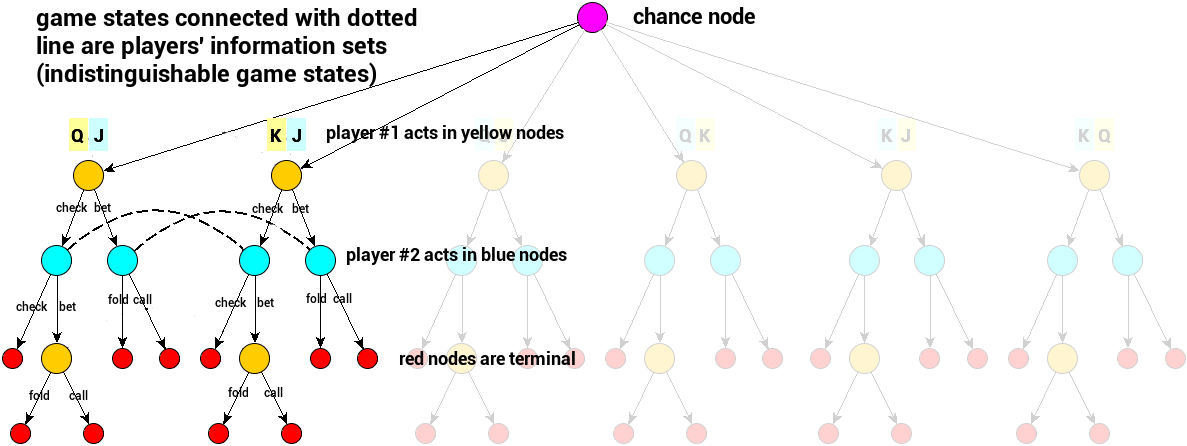
Please take a look at the game tree of Kuhn Poker – a simplified poker where only 3 different cards are dealt, there are no public cards, and only one private card for two players involved.Yellow nodes represent game states where player #1 acts, blue nodes represent game states where player #2 acts, edges represent actions and so transitions between game states.
Dotted lines connect information sets. In our example, two information sets for player 2 are presented. Blue player is not able to distinguish between nodes connected with single dotted line. He is only aware of the public action the yellow player performed and his private card J.
Purple chance node is a special type of node where no decision is made but some action is performed. In Kuhn Poker, there is only one chance node dealing the hands. In Texas Hold’em, these actions are initial hands or public cards dealings. The chance node has an interface similar to a ‘player node’ but it is not the decision point for any player – it is part of the game, an environment that happens to be random.
No regret learning
Before we take a look at the CFR itself, let’s focus on the main concept behind it: regret. That will lead us to no regret learning, which together with game theoretic implications, is a core of CFR.
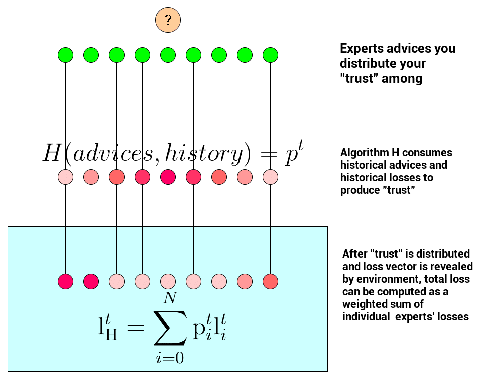
The concept of regret is central in problems of repeatedly making decisions in uncertain environments (also called online learning). To define it, let’s imagine we repeatedly (at consecutive times \( t \)) receive advice from \( N \) experts about a single phenomenon – like different predictions of the same stock price from \( N \) predefined Twitter accounts we monitor (don’t do it) or predictions of NBA games coming from our \( N \) predefined ‘hobby’ experts. After we receive the advice, our online algorithm \( \mathrm{H} \)’s goal is to distribute trust among experts or equivalently propose a probability distribution vector \( \mathrm{p}^t \) over \( N \) experts. After that, the environment (potentially adversarial) reacts and reveals the real outcome implying a loss vector \( \mathrm{l}^t \) that evaluates our \( N \) experts. The loss vector \( \mathrm{l}^t \) is a vector of size \( N \) that assigns losses for every single expert’s advice at time \( t \). Having a loss vector and our online algorithm’s ‘trust’ distribution, expected loss can be computed with:
\[\mathrm{l}_{\mathrm{H}}^t = \sum_{i=0}^N \mathrm{p}_i^t \mathrm{l}_i^t\]Now similarly, we can define a total loss for a single expert \( i \) to be
\[\mathrm{L}_\mathrm{i}^T = \sum_{t=0}^T \mathrm{l}_i^t\]Regret at time \( T \) is a difference between our algorithm’s total loss and the best single expert’s loss. Regret may be expressed via the following reflection:
If only I had listened to expert number \( i \) all the time, the total loss for his advice was the lowest…
It indeed expresses how much we regret not following the single best expert’s advice in all time steps.
Formally, regret is defined as follows:
\[\mathrm{R} = \mathrm{L}_{\mathrm{H}}^T - \min_i \mathrm{L}_\mathrm{i}^T\]Having defined the concept of regret, we can now introduce no-regret learning. We say that an online algorithm \( \mathrm{H} \) learns without regret if, in the limit (as \( T \) goes to infinity), its average regret goes to zero in the worst case – meaning no single expert is better than \( \mathrm{H} \) in the limit – there is no regret towards any single expert.
Regret matching as an example of a no-regret learning algorithm
There is a variety of online learning algorithms, but not all of them can be categorized as no-regret learning. In general, no deterministic online learning algorithm can lead to no-regret learning. If our algorithm \( \mathrm{H} \) produces a probability vector that places all probability mass on one expert, it won’t learn without regret. Randomization is necessary.
Here, we will take a closer look at one no-regret learning algorithm called Regret Matching, which borrows its update logic from the Polynomially Weighted Average Forecaster (PWA) (realized via certain hyper-parameter choice).
Regret Matching algorithm \( \hat{\mathrm{H}} \) will maintain the vector of weights assigned to experts. After the loss vector (again, representing consequences of our experts’ advice) is revealed, we can compute cumulative regret with respect to an expert \( i \) at time \( t \) (it expresses how we regret not listening to particular expert \( i \)):
\[\mathrm{R}_{i,t} = \mathrm{L}_{\hat{\mathrm{H}}}^t - \mathrm{L}_\mathrm{i}^t\]Having that, experts’ weights are updated with the formula:
\[w_{i,t} = (\mathrm{R}_{i,t})_+ = \max(0, \mathrm{R}_{i,t})\]and finally, components of our vector \( p^t \) in question (product of the algorithm) are given by:
\[p_i^t = \begin{cases} \dfrac{w_{i,t}}{\sum_{j \in N} w_{j,t}}, & \text{if } \sum_{j \in N} w_{j,t} > 0 \\ \dfrac{1}{N}, & \text{otherwise} \end{cases}\]Explanation:
Simply speaking, we observe all our experts and keep stats about their performance over time: positive cumulative regrets – \( N \) numbers (one for each expert) expressing how much we would gain if we switched from our current ‘trust’ distribution scheme and just listened to a single expert the whole time. As in the next round we don’t want to listen to experts that have negative cumulative regret (meaning we don’t regret not ‘listening’ to them), we omit it. Our ‘trust’ distribution vector \( p^t \) is then just the normalized version of \( w_t \) (or uniform if it does not make sense – when cumulative regret is non-positive for all experts). It indeed matches positive cumulative regret towards experts.
No-regret learning and game theory
Researchers have been studying no-regret learning in various different contexts. Interestingly, one particular no-regret learning algorithm called Hedge is a building block for Boosting and the AdaBoost algorithm for which Yoav Freund and Robert Schapire received the Gödel Prize in 2003. If you are interested in economical or financial contexts, you may want to have a look at Michael Kearns’ work.
A context that is particularly interesting for us is Game Theory. To start connecting no-regret learning and game theory, let’s consider the simple game of Rock-Paper-Scissors. We are going to abstract some details away so the whole thing matches the online learning framework. This will give us the ‘mandate’ to reason about no-regret learning in this setup.
Let’s assume players \( A \) and \( B \) are repeatedly playing a game of rock-paper-scissors.
From \( A \)’s point of view, he has to choose one action (rock, paper, or scissors) and play it. After both players act, payoffs can be calculated. From player \( A \)’s perspective again, payoff is a reward for playing an action of his choice, but in fact, nothing stops him from calculating rewards he would have been given for actions he has not played (freezing opponent’s move). Player \( A \) can then see the whole thing in the following way:
- Before he acts, he has 3 experts proposing one action each.
- When he acts, he in fact draws an action from a probability distribution over actions (experts/behavioral strategy).
- After that, the adversary presents a reward vector (depending on what the other player plays).
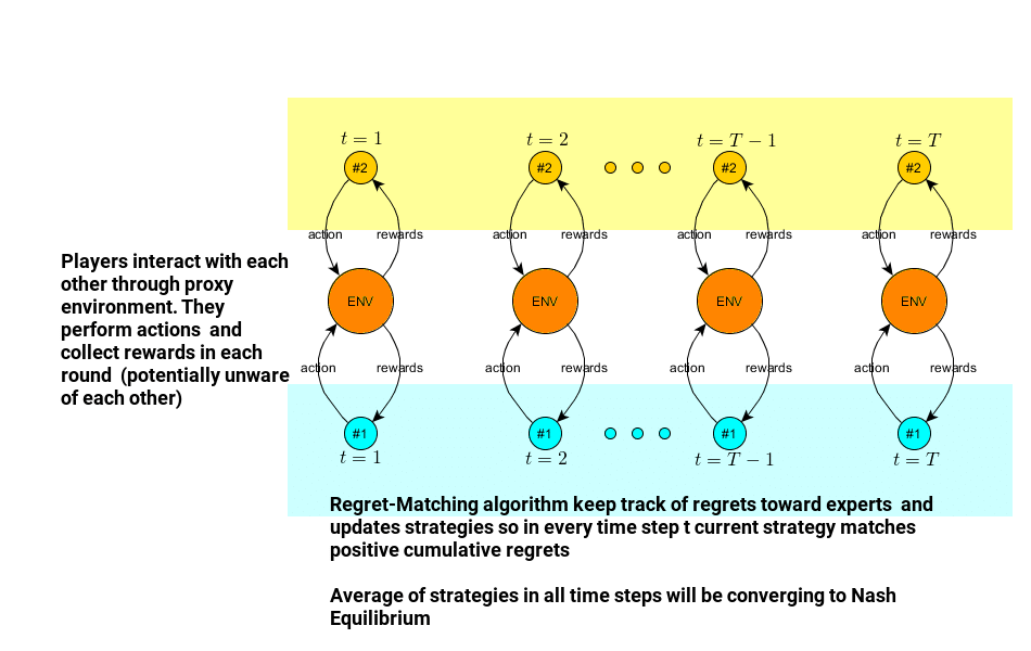
This is very similar to our online learning setup above. Now if we incorporate algorithm \( \mathrm{H} \) expressing how our player \( A \) learns ‘trust’ distribution among experts (or a behavioral strategy), we end up with almost the same model as in the previous section. The only subtle difference is that instead of costs, we receive rewards from the environment. But this can be easily handled by changing a sign and aggregate function (min → max) in the regret formulation.
Of course, our online-learning interpretation of a rock-paper-scissors game holds for other two-player zero-sum games.
Once we are in the online learning framework, we can ask: what will happen if both players adapt to one another via a no-regret learning algorithm \( \mathrm{H} \)? This question leads us to the following theorem:
Theorem:
If two no-regret algorithms play a zero-sum game against one another for \( T \) iterations with average regret less than \( \epsilon \), then their average strategies approximate Nash Equilibrium (up to \( 2\epsilon \)).
(A nice proof of this result can be found here.)
Average regret in the theorem is cumulative regret divided by time steps (number of game repetitions), and the average strategy is the mean of behavioral strategies used in every time step.
You may want to check out an example Python implementation of the Regret Matching algorithm for computing Rock-Paper-Scissors Nash Equilibrium here.
Average Overall Regret and Nash Equilibrium in extensive imperfect information games
In our considerations so far, we tried to compare our algorithm’s performance to the single best expert (action) over time. This led us to the notion of regret, no-regret learning, and its interesting relation to Nash Equilibrium. Comparing algorithm performance to the best single expert (action) was actually one of many possible choices; in general, we can think of so-called comparison classes. In the case of Rock-Paper-Scissors, we have just looked at one particular comparison class consisting of single actions only. But nothing stops us from studying other classes – like the class of behavioral or mixed strategies (probability distributions over actions).
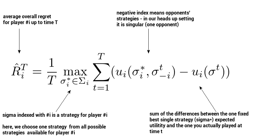
In fact, for Heads Up Texas Hold’em No-Limit Poker, it is beneficial to consider the set of mixed strategies as the comparison class. This leads us to the notion of average overall regret, where we regret not playing a particular mixed/behavioral strategy. If we consider repeatedly playing a game over time, we can think of average overall regret for player \( i \) at time \( T \) defined as:
It expresses how much we regret not playing a single fixed best response to all strategies our opponent played up until \( T \). Now, this type of regret is very handy because it leads to another very important fact:
Fact:
If both players play to minimize average overall regret, their average strategies will meet at an approximation of Nash Equilibrium at some point.
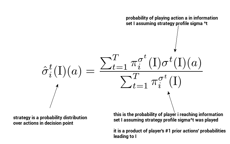
By average strategy in information set \( I \) for action \( a \) at time \( T \), we mean:
that is, a sum of all strategies played up to \( T \) in our information set weighted according to reach probabilities. Let’s keep this formula in mind because we will get back to it once we get to implementation.
The theorem depicted in green is very important for us here; later, it will turn out that counterfactual regret minimization is a ‘proxy’ minimizer of average overall regret and so leads to Nash Equilibrium.
Counterfactual regret minimization
Having the basics of game theory and no-regret learning, we can now move on to the main subject of this post: counterfactual regret minimization.
CFR was introduced in 2007 by Martin Zinkevich—nowadays a machine learning practitioner at Google, also the author of Rules of Machine Learning: Best Practices for ML Engineering.
Before we start looking at the formulas and interpreting them, please make sure you understand the difference between a game state (history) and an information set.
In essence, CFR is a regret-matching procedure applied to optimize an entity called immediate counterfactual regret, which, when minimized in every information set, is an upper bound on average overall regret (that we just learned about). Moreover, immediate counterfactual regret is guaranteed to go to zero in the limit if a regret-matching routine is applied. These two together imply that average overall regret can be minimized via counterfactual regret minimization. Minimizing average overall regret for both players leads to Nash Equilibrium, which in Heads-Up No Limit Texas Hold’em is a strategy that cannot be beaten in expectation!
CFR is defined with respect to these counterfactual versions of utility and regret. Let’s find out what that means.
Counterfactual utility
In one of the previous sections, we presented what expected utility means. We found out it is a convenient way of evaluating players’ strategies—here we will learn about another evaluation metric of players’ strategies, though this time our metric will be defined for every single information set separately. This metric is called counterfactual utility. We will learn why it has such a name in a moment.
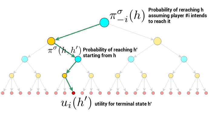
To begin in a math-less fashion, imagine you are at a particular decision point in Heads-Up NLTH poker. Of course, you are not aware of what cards your opponent holds. Let’s, for a moment, assume you decided to guess your opponent’s hand to be a pair of aces. That means you are no longer in an information set because you just put yourself in a specific game state (by assuming a particular opponent’s hand). That means you can compute expected utility for a subgame rooted in the game state you assumed. This utility would simply be:
\[\sum_{h' \in \mathrm{Z}} \pi^{\sigma}(h, h') u(h')\]where \( \pi^{\sigma}(h, h’) \) is the probability of reaching terminal game state \( h’ \) starting from \( h \), and \( \mathrm{Z} \) is the set of all terminal nodes (reach probabilities are products of all action probabilities prior to the current state, including chance). Please note that in this context, it is OK to consider all terminal nodes, as in practice only reachable nodes contribute to the sum because the probability of reaching unreachable nodes is zero.
If we make that assumption for every possible game state in our information set (every possible opponent’s hand), we will end up with a vector of utilities, one for each opponent’s hand. If we now weight these utilities according to probabilities of reaching these particular game states and add them together, we will end up having (a fraction of) regular expected utility.
To get counterfactual utility, we need to use another weighting scheme. For every opponent’s hand (game state \( h \)), let’s use the probability of reaching \( h \) assuming we wanted to get to \( h \). So instead of using our regular strategy from the strategy profile, we modify it a bit so it always tries to reach our current game state \( h \)—meaning that for each information set prior to the currently assumed game state, we pretend we always played pure behavioral strategy where the whole probability mass was placed in the action that was actually played and led to the current assumed state \( h \)—which is in fact counterfactual, in opposition to the facts, because we really played according to \( \sigma \). In practice, then, we just consider our opponent’s contribution to the probability of reaching the currently assumed game state \( h \). These weights (let’s call them counterfactual reach probabilities) express the following intuition: “how probable is it that my opponent gets here assuming I always played to get here?”
Counterfactual utility is then a weighted sum of utilities for subgames (each rooted in a single game state) from the current information set, with weights being normalized counterfactual probabilities of reaching these states.
Using normalized weighting scheme as described above for all subgames rooted in all game states in our information set leads to the formal definition of counterfactual utility.
Formally, counterfactual utility for information set \( \mathrm{I} \), player \( i \), and strategy \( \sigma \) is given by:
\[u_i(\sigma, \mathrm{I}) = \frac{\sum_{h \in \mathrm{I},\; h' \in \mathrm{Z}} \pi^{\sigma}_{-i}(h)\; \pi^{\sigma}(h, h')\; u(h') }{\pi_{-i}^{\sigma}(\mathrm{I})}\]The denominator is a sum of our counterfactual weights—a normalizing constant.
You may find an unnormalized form of the above—it is okay, and let’s actually have it too; it will come in handy later:
\[\hat{u}_i(\sigma, \mathrm{I}) = \sum_{h \in \mathrm{I},\; h' \in \mathrm{Z}} \pi^{\sigma}_{-i}(h)\; \pi^{\sigma}(h, h')\; u(h')\]Immediate Counterfactual Regret
To introduce counterfactual regret minimization, we will need to look at the poker game from a certain specific angle. First of all, we will be looking at a single information set, a single decision point. We will consider acting in this information set repeatedly over time with the goal to act in the best possible way with respect to a certain reward measure.
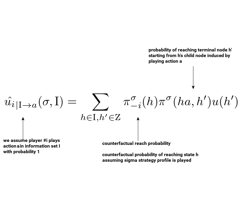
Assuming we are playing as player \( i \), let’s agree that the reward for playing action \( a \) is the unnormalized counterfactual utility under the assumption we played action \( a \) (let’s just assume this is how the environment rewards us). The entity in consideration is then defined as:
Please note that we replaced \( \pi^{\sigma}(h,h’) \) with \( \pi^{\sigma}(ha, h’) \) as we can discard the probability of going from \( h \) to \( ha \) where \( ha \) is the game state implied by playing action \( a \) in game state \( h \). We can do this because we assume we played \( a \) with probability 1.
We can easily abstract the whole thing as a ‘combining experts advice’ model via an interpretation similar to the Rock-Paper-Scissors game from the previous section:
- At our decision point, we have a fixed finite set of actions \( A(\mathrm{I}) \) (or experts’ advice).
- We assume we act in our information set \( \mathrm{I} \) according to some algorithm \( \mathrm{H} \) repeatedly over time.
- Algorithm \( \mathrm{H} \)’s job is to update probabilities of actions being played (behavioral strategy at our decision point).
- For every \( t \), we have a probability distribution over actions \( \sigma^t_{\mathrm{H}}(\mathrm{I}) \) that expresses our confidence of playing them (behavioral strategy/trust towards experts learned by \( \mathrm{H} \)).
- For every \( t \), a black-box mechanism (environment) triggers a reward vector being revealed (vector of unnormalized counterfactual utilities, one for each action, expressing consequences of playing these actions).
As you know already, in an online-learning setup it is beneficial to consider expected reward (and compare it to the single best action performance) of our algorithm \( \mathrm{H} \) over time. Let’s try to think about what expected reward we land on.
If we follow the expected reward definition and compute the weighted sum of the rewards vector using weights according to the behavioral strategy in our information set \( \mathrm{I} \) (a ‘trust’ distribution), we will actually end up having unnormalized counterfactual utility for \( \mathrm{I} \) at time \( t \):
\[\begin{align} \sum_{a \in A(\mathrm{I})} \sigma^t_{\mathrm{H}}(\mathrm{I})(a) \, \hat{u}_{|\mathrm{I} \rightarrow a}(\sigma^t_{\mathrm{H}}, \mathrm{I}) &= \\ \sum_{a \in A(\mathrm{I})} \sigma^t_{\mathrm{H}}(\mathrm{I})(a) \sum_{h \in \mathrm{I}, \, h' \in \mathrm{Z}} \pi^{\sigma^t_{\mathrm{H}}}_{-i}(h) \pi^{\sigma^t_{\mathrm{H}}}(ha, h') \, u(h') &= \\ \sum_{h \in \mathrm{I}, \, h' \in \mathrm{Z}} \pi^{\sigma^t_{\mathrm{H}}}_{-i}(h) \pi^{\sigma^t_{\mathrm{H}}}(h, h') \, u(h') &= \\ \hat{u}_i(\sigma^t_{\mathrm{H}}, \mathrm{I}) \end{align}\]Note that choosing action \( a \) gets \( \sigma^t_{\mathrm{H}}(\mathrm{I})(a) \) out of the formula but it is brought back again via the expected reward computation.
Having the total reward of algorithm \( \mathrm{H} \), we can define regret in our setting to be:
\[R_{i, \text{imm}}^T(\mathrm{I}) = \frac{1}{T} \max_{a \in A(\mathrm{I})} \sum_{t=1}^{T} \left( \hat{u}_{|\mathrm{I} \rightarrow a}(\sigma^t_{\mathrm{H}}, \mathrm{I}) - \hat{u}_i(\sigma^t_{\mathrm{H}}, \mathrm{I}) \right)\]which Zinkevich and his colleagues called Immediate Counterfactual Regret.
In some sense Immediate Counterfactual Regret is a standard regret we already learnt before. The difference here is the way we stretch things; previously for Rock-Paper-Scissors we represented the whole game as our decision-making problem with utility being our reward, here we are dealing with a single information set where unnormalized counterfactual utility (with one extra assumption) is a reward. The underlying idea is common for both cases – it is interpretation that differs.
Last important entity, Immediate Counterfactual Regret of not playing action \( a \) is given by:
\[R_{i, \text{imm}}^T(\mathrm{I}, a ) = \dfrac{1}{T} \sum_{t=1}^{T} \left( \hat{u_i}_{|\mathrm{I} \rightarrow a}(\sigma_{\mathrm{H}}^t, \mathrm{I}) - \hat{u}_i(\sigma_{\mathrm{H}}^t, \mathrm{I}) \right)\]and is actually equivalent to regret of not listening to expert \( a \) in our no-regret interpretation.
Immediate Counterfactual Regret and Nash Equilibrium
Landing in regret minimization framework again does not imply we can apply our theorem that we used for Rock-Paper-Scissors. The difference is that in our case we ‘regret’ in the single information set only, not the whole game. Fortunately, Zinkevich and his colleagues showed that this is still OK and we can still land in Nash Equilibrium if we consecutively apply regret matching for Immediate Counterfactual Regret over time for all information sets. They actually proved two things:
- For fixed strategy profile, if we compute immediate counterfactual regrets in all information sets, their sum will bound overall average regret.
- If the player selects actions according to the regret matching routine, counterfactual regret goes to zero eventually.
This means you can apply regret matching to all information sets simultaneously for both players, and you will end up minimizing all of them and so minimizing average overall regret – and that actually means you will end up in Nash Equilibrium.
Counterfactual Regret Minimization – Implementation Plan
Let’s try to summarize what we actually need to compute Nash Equilibrium via counterfactual regret minimization.
From a very high-level point of view, we will need to:
- Initialize strategies for both players – uniform distribution is okay.
- Run the regret matching routine for all information sets for both players separately. Each time, we will assume there is an unknown adversary environment players may not be aware of, and they just try to play the best they can via application of no-regret learning in every time step. It means they will be adjusting their current strategy in the current information set so it matches total positive regret (which happens to be counterfactual regret as we already established).
- Consecutive application of no-regret learning for both players for all information sets will trigger lots of strategy changes over time. Following our theorem, the averages of these strategies for both players will be an approximation of Nash Equilibrium.
The Memory Requirements
In every single information set \( \mathrm{I} \), the regret matching routine requires us to distinguish:
-
Reward for playing action \( a \) at time \( t \):
\[\hat{u_i}^t_{|\mathrm{I} \rightarrow a}(\sigma^t, \mathrm{I}) = \sum_{h \in \mathrm{I},\ h' \in \mathrm{Z}} \pi^{\sigma^t}_{-i}(h) \pi^{\sigma^t}(ha, h') u(h')\]Every action will be rewarded via unnormalized counterfactual utility assuming action was played. It is worth noting every element of the sum above can be computed separately for every game state in the information set:
\[\hat{u_i}^t_{|\mathrm{I} \rightarrow a}(\sigma^t, h) = \pi^{\sigma^t}_{-i}(h) \sum_{h' \in \mathrm{Z}} \pi^{\sigma^t}(ha, h') u(h')\]Let’s remember that, in fact, later on in our actual implementation, we will be traversing through game states, not information sets.
-
Total reward for playing action \( a \) up to time \( T \):
\[\sum_{t=1}^T \hat{u_i}^t_{|\mathrm{I} \rightarrow a}(\sigma^t, \mathrm{I})\] -
Reward for playing according to current behavioral strategy at time \( t \):
\[\hat{u}_i(\sigma^t, \mathrm{I}) = \sum_{h \in \mathrm{I},\ h' \in \mathrm{Z}} \pi^{\sigma^t}_{-i}(h) \pi^{\sigma^t}(h, h') u(h')\]This will express how our current strategy performs in terms of unnormalized counterfactual utility at time \( t \).
-
Total reward for playing according to our behavioral strategies up to time \( T \):
We will compare this value with total rewards for playing each action and update the strategy for the next iteration accordingly.
Regret matching routine will update a strategy at time \( t \) in information set \( \mathrm{I} \) with the following formula:
\[\sigma^{T+1}_\mathrm{H} (\mathrm{I})(a) = \begin{cases} \dfrac{R_{i, \text{imm}}^{T,+}(\mathrm{I}, a )}{\displaystyle\sum_{a' \in \mathrm{I}} R_{i, \text{imm}}^{T,+}(\mathrm{I}, a')},& \text{if } \displaystyle\sum_{a' \in \mathrm{I}} R_{i, \text{imm}}^{T,+}(\mathrm{I}, a') > 0 \\[2ex] \dfrac{1}{T}, & \text{otherwise} \end{cases} =\]where
\[R_{i, \text{imm}}^T(\mathrm{I}, a ) = \dfrac{1}{T} \sum_{t=1}^{T} \left( \hat{u_i}_{|\mathrm{I} \rightarrow a}(\sigma^t_{\mathrm{H}}, \mathrm{I}) – \hat{u}_i(\sigma^t_{\mathrm{H}}, \mathrm{I}) \right)\]In every iteration, we need current strategy profile, game tree (this is static), and immediate counterfactual regrets. An important observation here is that we don’t really need \( \dfrac{1}{T} \) in \( R_{i, \text{imm}}^{T,+} \) because it cancels out anyway. Therefore, for every information set and every action, it is enough to store the following sum, let’s call it \( R_{i, \text{cum}}^T(\mathrm{I}, a ) \):
\[R_{i, \text{cum}}^T(\mathrm{I}, a ) = \sum_{t=1}^{T} \left( \hat{u_i}_{|\mathrm{I} \rightarrow a}(\sigma^t_{\mathrm{H}}, \mathrm{I}) – \hat{u}_i(\sigma^t_{\mathrm{H}}, \mathrm{I}) \right)\]Memory-wise we only need current behavioral strategy profile \( \sigma_t \) and vector of \( R_{i, \text{cum}}^T(\mathrm{I}, a ) \) for every information set to perform our updates in consecutive iterations.An additional entity we need is sum of all strategies up till now for every information set. This is needed because, at the very end, we plan to average all strategies to compute our ultimate goal: Nash Equilibrium.
Computation – What Do We Need to Compute to Get Nash Equilibrium?
We already established that for every information set, in every iteration, we will need to store three vectors: vector of sums of strategies played so far, vector of \( R_{i, \text{cum}}^T(\mathrm{I}, a ) \), and current strategy \( \sigma_t \).
Now we need a clever way to go to every possible information set, compute counterfactual utilities for every action, counterfactual utility for our behavioral strategy, add the difference between these two up to the vector of cumulative immediate regrets, and finally compute the strategy for the next iteration.
The very core entity we need in order to achieve so is game-state centric unnormalized counterfactual utility (under assumption that action \( a \) was played):
\[\hat{u_i}^t_{|\mathrm{I} \rightarrow a}(\sigma^t, h) = \pi^{\sigma^t}_{-i}(h) \sum_{h' \in \mathrm{Z}} \pi^{\sigma^t}(ha, h') u(h')\]If we had it computed for all actions and game states in information set \( \mathrm{I} \), we could easily derive the rest of the entities involved. This is a clue of how we need our final algorithm to be constructed.
Let’s then focus on how we could cleverly compute these values assuming we have the strategies for both players in place. We will start by introducing a notion of expected utility in a game state:
\[u_i^{\sigma}(h) = \sum_{h' \in \mathrm{Z}} \pi^{\sigma}(h, h') u_i(h')\]If this was computed for the root of the game tree, it would result in the expected utility of the game – a well-known concept in game theory. We will now proceed in the following way: we will start with the expected utility computation algorithm and add more and more side effects to get our final CFR algorithm.
(The code in the following section is a pseudo-code, some unimportant details are hidden. To see the full working example of CFR, please take a look at the repository here).
Expected utility computation is as easy as recursive tree traversal + propagating the results back:
1
2
3
4
5
6
7
8
9
10
def _utility_recursive(self, state):
    if state.is_terminal():
        # Evaluate terminal node according to the game result
        return state.evaluation()
    # Sum up all utilities for playing actions in our game state
    utility = 0.
    for action in state.actions:
        # Utility computation for current node, here we assume sigma is available
        utility += self.sigma[state.inf_set()][action] * self._utility_recursive(state.play(action))
    return utility
(We assume chance nodes have an interface similar to regular game states).
There is actually only a very subtle difference between our unnormalized counterfactual utility and the expected utility. In fact, our expected utility can be seen as a sum of the following:
\[\sigma(h)(a) \sum_{h' \in \mathrm{Z}} \pi^{\sigma}(ha, h') u_i(h')\]for every action \( a \) available in \( h \). The only difference is the weighting component. In the case of unnormalized counterfactual utility, we use counterfactual reach probability; in the case of expected utility, it is the transition probability between game states. Let’s then try to inject some extra code, a side effect, into the utility computation algorithm to get unnormalized counterfactual utilities:
1
2
3
4
5
6
7
8
9
10
11
12
13
14
def _cfr_utility_recursive(self, state):
    if state.is_terminal():
        # Evaluate terminal node according to the game result
        return state.evaluation()
    # Sum up all utilities for playing actions in our game state
    utility = 0.
    for action in state.actions:
        child_state_utility = self._cfr_utility_recursive(state.play(action))
        # Utility computation for current node, here we assume sigma is available
        utility += self.sigma[state.inf_set()][action] * child_state_utility
        # Computing counterfactual utilities as a side effect, we assume we magically have cfr_reach function here
        cfr_utility[action] = cfr_reach(state.inf_set()) * child_state_utility
    # Function still returns utility, side effect was added to compute counterfactual utility too
    return utility
By adding this tiny side effect to our utility computation routine, we are now computing unnormalized counterfactual utilities for every possible action \( a \) in \( h \) for the whole game tree (if started from the root)!
One puzzle that is still missing is the weighting component (counterfactual reach probability), the probability of our opponent getting to \( h \) under the assumption we did all we could to get there. Good news is that these probabilities are products of transition probabilities between states we already visited. It means we must be able to collect these products on our way down to the current game state.
1
2
3
4
5
6
7
8
9
10
11
12
13
14
15
16
17
18
19
20
def _cfr_utility_recursive(self, state, reach_a, reach_b):
    if state.is_terminal():
        # Evaluate terminal node according to the game result
        return state.evaluation()
    # Sum up all utilities for playing actions in our game state
    utility = 0.
    for action in state.actions:
        child_reach_a = reach_a * (self.sigma[state.inf_set()][action] if state.to_move == A else 1)
        child_reach_b = reach_b * (self.sigma[state.inf_set()][action] if state.to_move == B else 1)
        child_state_utility = self._cfr_utility_recursive(state.play(action), child_reach_a, child_reach_b)
        # Utility computation for current node, here we assume sigma is available
        utility += self.sigma[state.inf_set()][action] * child_state_utility
        children_states_utilities[action] = child_state_utility
    cfr_reach = reach_b if state.to_move == A else reach_a
    for action in state.actions:
        # Player to act is either 1 or -1
        # Utilities are computed for player 1 - therefore we need to change their signs if player #2 acts
        action_cfr_regret = state.to_move * cfr_reach * children_states_utilities[action]
    # Function still returns utility, side effect was added to compute counterfactual utility too
    return utility
We added extra parameters to our function; now, at every game state, we keep track of counterfactual reach probabilities for both players. They are products of probabilities of actions that were played prior to the current game state (computed separately for both players).
All we need now is to run our routine for the game tree root node with reach probabilities equal to 1 for both players. This will cause counterfactual utility of not playing actions being available. Now we need to inject the rest of the code:
1
2
3
4
5
6
7
8
9
10
11
12
13
14
15
16
17
18
19
20
21
22
23
24
25
26
27
28
29
30
31
def _cfr_utility_recursive(self, state, reach_a, reach_b):
    children_states_utilities = {}
    if state.is_terminal():
        # Evaluate terminal node according to the game result
        return state.evaluation()
    # Please note that now we also handle chance node, we simply traverse the tree further down
    # not breaking computation of utility
    if state.is_chance():
        outcomes = {state.play(action) for action in state.actions}
        return sum([state.chance_prob() * self._cfr_utility_recursive(c, reach_a, reach_b) for c in outcomes])

    # Sum up all utilities for playing actions in our game state
    utility = 0.
    for action in state.actions:
        child_reach_a = reach_a * (self.sigma[state.inf_set()][action] if state.to_move == A else 1)
        child_reach_b = reach_b * (self.sigma[state.inf_set()][action] if state.to_move == B else 1)
        child_state_utility = self._cfr_utility_recursive(state.play(action), child_reach_a, child_reach_b)
        # Utility computation for current node, here we assume sigma is available
        utility += self.sigma[state.inf_set()][action] * child_state_utility
        children_states_utilities[action] = child_state_utility
    (cfr_reach, reach) = (reach_b, reach_a) if state.to_move == A else (reach_a, reach_b)
    for action in state.actions:
        # Player to act is either 1 or -1
        # Utilities are computed for player 1 - therefore we need to change their signs if player #2 acts
        action_cfr_regret = state.to_move * cfr_reach * (children_states_utilities[action] - utility)
        # We start accumulating cfr_regrets for not playing actions in information set
        # and action probabilities (weighted with reach probabilities) needed for final NE computation
        self._cumulate_cfr_regret(state.inf_set(), action, action_cfr_regret)
        self._cumulate_sigma(state.inf_set(), action, reach * self.sigma[state.inf_set()][action])
    # Function still returns utility, side effect was added to compute counterfactual utility too
    return utility
We added a few important bits; first of all, now we cumulate unnormalized counterfactual utilities for actions in information sets, and we sum up sigmas (to later on compute NE out of it). Also, we handle chance nodes – simply by omitting CFR-specific side effects (we don’t make decisions in chance nodes – no need to compute anything) trying not to break utility computation.
Running this once with reach for both players being 1 will result in accumulating strategies and unnormalized counterfactual regrets in all information sets and actions. After such an iteration, we have to update sigma for the next iteration via the regret matching routine:
1
2
3
4
5
6
7
8
9
10
11
12
13
14
15
16
def __update_sigma_recursively(self, node):
    # Stop traversal at terminal node
    if node.is_terminal():
        return
    # Omit chance nodes
    if not node.is_chance():
        self._update_sigma(node.inf_set())
    # Go to subtrees
    for k in node.children:
        self.__update_sigma_recursively(node.children[k])

def _update_sigma(self, i):
    rgrt_sum = sum(filter(lambda x: x > 0, self.cumulative_regrets[i].values()))
    nr_of_actions = len(self.cumulative_regrets[i].keys())
    for a in self.cumulative_regrets[i]:
        self.sigma[i][a] = max(self.cumulative_regrets[i][a], 0.) / rgrt_sum if rgrt_sum > 0 else 1. / nr_of_actions
That leads us to a function:
1
2
3
4
5
6
def run(self, iterations=1):
    for _ in range(iterations):
        self._cfr_utility_recursive(self.root, 1, 1)
        # Since we do not update sigmas in each information set while traversing, we need to
        # traverse the tree to update it now
        self.__update_sigma_recursively(self.root)
After running our run method, we are ready to compute Nash Equilibrium (in a manner similar to new sigma):
1
2
3
4
5
6
7
8
9
10
11
12
13
14
15
def compute_nash_equilibrium(self):
    self.__compute_ne_rec(self.root)

def __compute_ne_rec(self, node):
    if node.is_terminal():
        return
    i = node.inf_set()
    if node.is_chance():
        self.nash_equilibrium[i] = {a: node.chance_prob() for a in node.actions}
    else:
        sigma_sum = sum(self.cumulative_sigma[i].values())
        self.nash_equilibrium[i] = {a: self.cumulative_sigma[i][a] / sigma_sum for a in node.actions}
    # Go to subtrees
    for k in node.children:
        self.__compute_ne_rec(node.children[k])
One iteration of counterfactual regret minimization turns out to be a single pass through the game tree plus another pass for sigma and Nash equilibrium computations. In essence, it is a utility computation routine with some side effects added.
Going through the whole game tree a few times should already raise a red flag. For large-size game trees, it is very impractical.
Reducing Game Tree Size via Chance Sampling
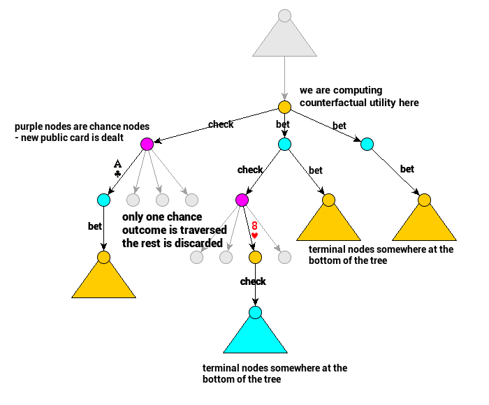
Zinkevich and colleagues decided to limit the number of visited nodes by sampling only one chance outcome at a time. This means they do not visit all information sets in a single iteration. They explore all possible actions in the information sets they visit though.
In the case of poker, sampling each chance node only once means that every single information set contains only one game state. That is because also initial hand dealing is sampled only once, and the whole tree traversal is performed for that one hand only. This means we only consider a single hand in an information set. That implies sigma can be updated right after computing regret in a game state – we don’t need an additional traverse to update it.
Let’s improve our implementation then. Whenever we end up in a chance node, we need to sample one outcome and follow that choice without changing reach probabilities; we just continue traversal ‘normally’ returning utility for the chosen chance outcome. Another bit is adding sigma update at the end of the ‘node visit’ – we can do it because this is the only time we are there for a single iteration.
1
2
3
4
5
6
7
8
9
10
11
12
13
14
15
16
17
18
19
20
21
22
23
24
25
26
27
28
def _cfr_utility_recursive(self, state, reach_a, reach_b):
    if state.is_terminal():
        # Evaluate terminal node according to the game result
        return state.evaluation()
    # Now we only go through a single outcome of chance
    if state.is_chance():
        return self._cfr_utility_recursive(state.sample_one(), reach_a, reach_b)

    # Sum up all utilities for playing actions in our game state
    utility = 0.
    for action in state.actions:
        child_state_utility = self._cfr_utility_recursive(state.play(action))
        # Utility computation for current node, here we assume sigma is available
        utility += self.sigma[state.inf_set()][action] * child_state_utility
        children_states_utilities[action] = child_state_utility
    (cfr_reach, reach) = (reach_b, reach_a) if state.to_move == A else (reach_a, reach_b)
    for action in state.actions:
        # Player to act is either 1 or -1
        # Utilities are computed for player 1 - therefore we need to change their signs if player #2 acts
        action_cfr_regret = state.to_move * cfr_reach * (children_states_utilities[action] - utility)
        # We start accumulating cfr_regrets for not playing actions in information set
        # and action probabilities (weighted with reach probabilities) needed for final NE computation
        self._cumulate_cfr_regret(state.inf_set(), action, action_cfr_regret)
        self._cumulate_sigma(state.inf_set(), action, reach * self.sigma[state.inf_set()][action])
    # Sigma update can be performed here now as any information set contains a single game state
    self._update_sigma(state.inf_set())
    # Function still returns utility, side effect was added to compute counterfactual utility too
    return utility
Sampling makes a single iteration much faster but may require more iterations than the vanilla version of CFR.
In practice, people often use other versions of CFR. One particularly intriguing improvement is an algorithm called CFR+ (one that was used in Cepheus). CFR+ is especially nice because it does not require the averaging step (which costs the whole tree traversal) to get Nash Equilibrium. After each iteration, sigma is already its good approximation. Interestingly, it was never proved why sigma is enough, but it tends to happen in practice very often.
The final code for this post – our example toy CFR with chance sampling implementation – is available on GitHub. It may differ a bit from the pseudo-code presented above but should be more or less readable.
Summary
That’s all, folks.
I hope you enjoyed this (a bit too long) tutorial and you are now more familiar with the basics of game theory, no-regret learning, and counterfactual regret minimization. Hopefully, you can implement a simple version of CFR for yourself or maybe even extend existing ones.
Good luck with your projects and have a good rest of the day (+ lots of nice hands)!


