Bellman Equations, Dynamic Programming and Reinforcement Learning (part 1)
Reinforcement learning has been on the radar of many, recently. It has proven its practical applications in a broad range of fields: from robotics through Go, chess, video games, chemical synthesis, down to online marketing. While being very popular, Reinforcement Learning seems to require much more time and dedication before one actually gets any goosebumps. Playing around with neural networks with PyTorch for an hour for the first time will give instant satisfaction and further motivation. Similar experience with RL is rather unlikely. If you are new to the field, you are almost guaranteed to have a headache instead of fun while trying to break in.
One attempt to help people breaking into Reinforcement Learning is OpenAI SpinningUp project – a project aiming to help taking first steps in the field. There is a bunch of online resources available too: a set of lectures from Deep RL Bootcamp and the excellent Sutton & Barto book.
What is this series about
This blog post series aims to present the very basic bits of Reinforcement Learning: Markov Decision Process model and its corresponding Bellman equations, all in one simple visual form.
To get there, we will start slowly by introducing an optimization technique proposed by Richard Bellman called dynamic programming. Then we will take a look at the principle of optimality: a concept describing a certain property of the optimization problem solution that implies dynamic programming being applicable via solving corresponding Bellman equations. All will be guided by an example problem of maze traversal.
Dynamic programming
The term ‘dynamic programming’ was coined by Richard Ernest Bellman, who in the very early 50s started his research about multistage decision processes at RAND Corporation, at that time fully funded by the US government. Bellman’s RAND research being financed by tax money required solid justification. Funding seemingly impractical mathematical research would be hard to push through. Richard Bellman, in the spirit of applied sciences, had to come up with a catchy umbrella term for his research. He decided to go with dynamic programming because these two keywords combined – as Richard Bellman himself said – was something not even a congressman could object to.

Principle of optimality
An optimal policy has the property that, whatever the initial state and the initial decision, the remaining decisions must constitute an optimal policy with regard to the state resulting from the first decision.
Richard Bellman
DP is all about multistage decision processes with terminology floating around terms such as policy, optimal policy or expected reward making it very similar to Reinforcement Learning which in fact is sometimes called approximate dynamic programming.
At the time he started his work at RAND, working with computers was not really everyday routine for a scientist – it was still very new and challenging. An applied mathematician had to slowly start moving away from classical pen and paper approach to more robust and practical computing. Therefore he had to look at the optimization problems from a slightly different angle; he had to consider their structure with the goal of how to compute correct solutions efficiently.
In RAND Corporation, Richard Bellman was facing various kinds of multistage decision problems. In a report titled Applied Dynamic Programming, he described and proposed solutions to lots of them including:
- Resources allocation problem (present in economics)
- The minimum time-to-climb problem (time required to reach optimal altitude-velocity for a plane)
- Computing Fibonacci numbers (common hello world for computer scientists)
- Controlling nuclear reactor shutdown
One of his main conclusions was that multistage decision problems often share common structure. That led him to propose the principle of optimality – a concept expressed with equations that were later called after his name: Bellman equations.
Simple example of dynamic programming problem
To understand what the principle of optimality means and so how corresponding equations emerge, let’s consider an example problem. Imagine an agent enters the maze and its goal is to collect resources on its way out. The objective in question is the amount of resources the agent can collect while escaping the maze.
Let’s take a look at the visual representation of the problem below:
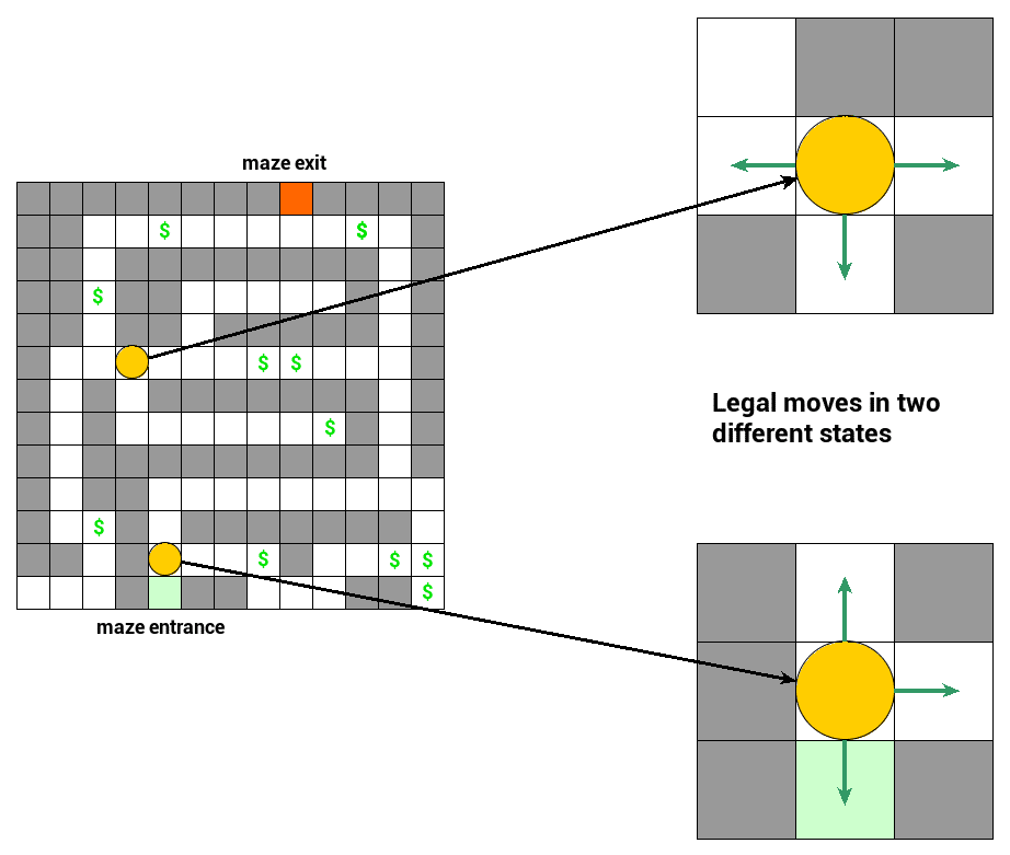
- Yellow circles represent current state – location of our agent
- Green arrows are called actions (moves, decisions). An action, when applied to a state, transforms it to another state. Our transitions are fully deterministic – once you choose an action you always end up in the same resulting state
- Green square represents the maze entrance location; this is where our agent starts moving
- Red square represents the maze exit location where our agent wants to get
- Dollar sign represents additional resource bonus agent collects on the way out from the maze
Plus a few rules to make it more precise:
- Our agent starts at maze entrance and has limited number of $N = 100$ moves before reaching a final state
- Our agent is not allowed to stay in the current state. The only exception is the exit state where the agent will stay once it’s reached
- Reaching a state marked with a dollar sign is rewarded with $k = 4$ resource units
- Minor rewards are unlimited, so the agent can exploit the same dollar sign state many times
- Reaching a non-dollar sign state costs one resource unit (you can think of fuel being burnt)
- Reaching the maze exit is rewarded with $l = 1000$ resource units. Once it’s reached, there is no way back to the maze – in practice, we could achieve this by adding an extra state that the agent goes to and stays at once the exit is reached
- As a consequence of 6, collecting the exit reward can happen only once
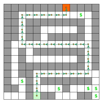
This loose formulation yields a multistage decision optimization problem where every possible sequence of 100 moves is a solution candidate. Such a solution candidate is also what is often called a policy (or a plan). Every policy can be evaluated – simply by traversing through the maze with respect to the policy details. In our case, evaluation is expressed as the amount of resources the agent collects on his way out. Our job then is to find an optimal policy evaluation or – in other words – find out what is the maximum amount of resources the agent can collect after $N$ moves.
Let’s describe all the entities we need and write down relationships between them.
First of all, we are going to traverse through the maze, transiting between states via actions (decisions). When an action is performed in a state, our agent will change its state. Let’s write it down as a function $f$ such that $f(s, a) = s’$, meaning that performing action $a$ in state $s$ will cause the agent to move to state $s’$.
In every state, we will be given an instant reward. Its value will depend on the state itself, all rewarded differently. We can then express it as a real function $r(s)$.
We also need a notion of a policy: a predefined plan of how to move through the maze. Let’s denote policy by $\pi$ and think of it as a function consuming a state and returning an action: $\pi(s) = a$. Policies that are fully deterministic are also called plans (which is the case for our example problem).
Once we have a policy, we can evaluate it by applying all actions implied while maintaining the amount of collected/burnt resources.
Another important bit is that among all possible policies there must be one (or more) that results in the highest evaluation; this one will be called an optimal policy. The optimal policy is also a central concept of the principle of optimality.
The principle of optimality
The principle of optimality is a statement about a certain interesting property of an optimal policy. The principle of optimality states that if we consider an optimal policy, then the subproblem yielded by our first action will have an optimal policy composed of remaining optimal policy actions.
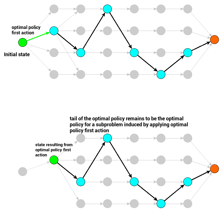
- Black arrows represent a sequence of optimal policy actions – the one that is evaluated with the greatest value.
- Green arrow is the optimal policy’s first action (decision) – when applied, it yields a subproblem with a new initial state. The principle of optimality is related to this subproblem’s optimal policy.
- Green circle represents the initial state for a subproblem (the original one or the one induced by applying the first action)
- Red circle represents the terminal state – assuming our original parametrization, it is the maze exit
Bellman equations
For a policy to be optimal means it yields the optimal (best) evaluation $v^N_*(s_0)$. Therefore, we can formulate the optimal policy evaluation as:
\[v^N_*(s_0) = \max_{\pi} v^N_\pi(s_0)\]Which is already a clue for a brute force solution. Just iterate through all of the policies and pick the one with the best evaluation. But we want it a bit more clever. Assuming $s’$ to be a state induced by the first action of policy $\pi$, the principle of optimality lets us re-formulate it as:
\[v^N_*(s_0) = \max_{\pi} \{ r(s') + v^{N-1}_*(s') \}\]Because $v^{N-1}_*(s’)$ is independent of $\pi$ and $r(s’)$ only depends on its first action, we can reformulate our equation further:
\[v^N_*(s_0) = \max_{a} \{ r(f(s_0, a)) + v^{N-1}_*(f(s_0, a)) \}\]This equation, implicitly expressing the principle of optimality, is also called the Bellman equation.
Bellman equation does not have exactly the same form for every problem. The way it is formulated above is specific for our maze problem. What is common for all Bellman Equations though is that they all reflect the principle of optimality one way or another.
There are some practical aspects of Bellman equations we need to point out:
- For deterministic problems, expanding Bellman equations recursively yields problem solutions – this is in fact what you may be doing when you try to compute the shortest path length for a job interview task, combining recursion and memoization.
- Given optimal values for all states of the problem, we can easily derive the optimal policy (policies) simply by going through our problem starting from the initial state and always greedily choosing actions to land in a state of the highest value.
- Knowledge of an optimal policy $\pi$ yields the value – that one is easy, just go through the maze applying your policy step by step counting your resources.
Summary
This post presented very basic bits about dynamic programming (being background for reinforcement learning which nomen omen is also called approximate dynamic programming). In the next post, we will try to present a model called Markov Decision Process which is a mathematical tool helpful to express multistage decision problems that involve uncertainty. This will give us a background necessary to understand RL algorithms.
Tags: bellman equation, machine learning, reinforcement learning