Random walk vectors for clustering (final)

Hi there. I have finally managed to be finishing the long series of posts about how to use random walk vectors for clustering problem. It’s been a long series and I am happy to finish it as the whole blog suddenly moved away from being about Julia and turned into a random walk weirdo… Anyways let’s finish what has been started.

In the previous post we saw how to use many random walks to cluster given dataset. Presented approach was evaluated on toy datasets and our goal for this post is to try it on some more serious one. We will then apply same approach onto MNIST dataset—a set of handwritten digits images. We will compare the results to the state-of-the art k-means algorithm.

For a reminder of what is going to be applied – please take a step back to the previous post.

Ok, let’s start. The very first step is to load the MNIST dataset and prepare it. Julia comes with a package that contains the dataset we want to play with. It is called MNIST and can be installed and loaded with:

Pkg.Add("MNIST")
using MNIST

Load the dataset with

points, labels = testdata()

Next step of the preprocessing is to apply Restricted Boltzmann Machines to reduce data dimensionality. That is quite easy too. Without going into details let’s just blindly apply it. Boltzmann package will help us:

using Boltzmann
points = points ./ (maximum(points) - minimum(points))
m = BernoulliRBM(28*28, 40)
fit(m, points, n_iter=24)
data_matrix = transform(m, points)

First we normalize the dataset and then apply reduction to end up with data_matrix variable holding new reduced dataset (of dimensionality 40).

We will now do simple experiment. We will run the algorithm 100 times for each parameter setup. Parameters in this case are: number of random walks and number of vectors. We will then go through some points of parameter space and for each point run 100 experiments. Single experiment is then evaluated using varinfo function from package Clustering. Then we will run k-means (again 100 times) on the same data and compare varinfo metric between k-means and random walk based clustering. Let’s start with the first part then:

similarity_matrix = compose_similarity_matrix(data_matrix, 1.)
P = compose_random_walk_matrix(similarity_matrix)
walks = [1,2,3,4,6,8,12,16]
vectors = [50,100,300,500,1000]
experiments = 100
results = zeros(length(walks), length(vectors), experiments)

for i = 1:length(walks)
  walk = walks[i]
  P_powered = P^walk
  for j = 1:length(vectors)
    vect = vectors[j]
    for k = 1:experiments
      N = size(P_powered,1)
      v = zeros(size(P,1), vect)
      seed = choose_seed(N, (1./N) * ones(size(P_powered,1), 1))
      v[:,1] = P_powered[:, seed]
      for l = 2:vect
        seed = choose_seed(N, v)
        @inbounds v[:,l] = P_powered[:, seed]
      end
      cluster_membership = nmf_clustering(v, 10)
      result = varinfo(10000, int(labels[:] + 1), 10000, int(cluster_membership[:]))
      results[i,j,k] = result
    end
  end
end

Let’s now compute mean of all experiments for given parameters set:

results_mean = mean(results, 3)[:, :, 1]

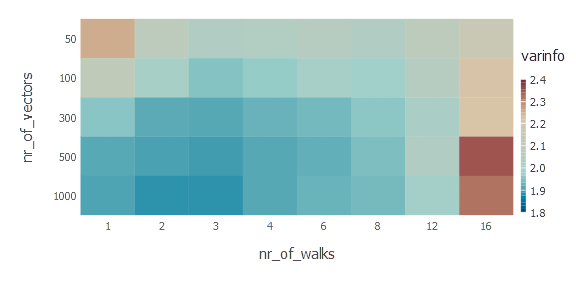
and display it to see what parameters work best (with respect to the metric of our choice):

using Gadfly 
using DataFrames
nr_of_walks, nr_of_vectors, values = findnz(results_mean)
function walks_label(x) walks[x] end
function vectors_label(x) vectors[x] end
plot(
  DataFrame(nr_of_walks = nr_of_walks, nr_of_vectors = nr_of_vectors, varinfo = values), 
  x="nr_of_walks", y="nr_of_vectors",
  color="varinfo",
  Coord.cartesian(yflip=true),
  Scale.color_continuous(),
  Scale.x_discrete(labels=walks_label),
  Scale.y_discrete(labels=vectors_label),
  Geom.rectbin,
  Stat.identity
)

Let’s quickly interpret the results we see. First of all—the more random walk vectors the better. Second observation is that there exists optimal steps of random walk. In this case we have 3 random walk steps producing best results. It makes sense, of course. Probability diffusion makes sense here only to some extent, in fact at some point it converges to trivial stationary distribution.

One last evaluation is a sanity check and comparison with k-means algorithm. Again we will use implementation from Clustering package.

v = zeros(100)
for i = 1:100
    k = kmeans(data_matrix, 10)
    v[i] = varinfo(10, int(labels) + 1, 10, k.assignments)
end
print(mean(v))

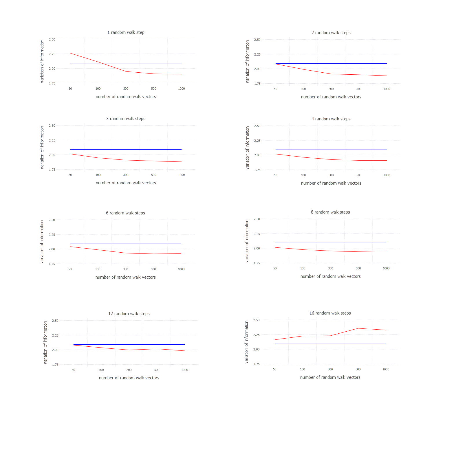
After running k-means 100 times average varinfo metric is 2.12 in case of my experiment. Let’s see how it relates to the results derived from random walk based clustering. Let’s plot how variation of information changes with number of vectors for given number of random walk steps.

plot(
  layer(x = vectors, y = mean(data, 3)[1, :, 1][:], Geom.line, Theme(default_color=color("red"))),
  layer(x = vectors, y = fill(mean(v), 5), Geom.line, Theme(default_color=color("blue"))),
  Guide.title("1 random walk step"),
  Guide.xlabel("number of random walk vectors"),
  Guide.ylabel("variation of information"),
  Scale.x_discrete()
)

Results for every possible setting look like below [blue === k-means; red === random walk clustering]:

Conclusions

Despite obvious desperate need for optimization (not powering the matrix to n-th + similarity matrix sparsification) solution seems to beat k-means in that one specific case for given subset of parameters. Obviously some of the problems remain unsolved like how to choose parameter when composing similarity matrix. If it is not chosen properly the approach may be useless. Anyways, it was possible to run a long experiment in Julia without any problems and it was quite fast without any big effort of mine. Next post I will try to play with neural networks a bit, implementing backpropagation algorithm.

---

Author: int8

Tags: clustering, Consensus clustering, non negative matrix factorization, random walk, restricted boltzmann machines